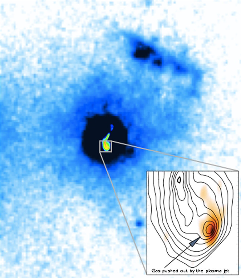
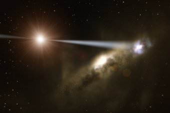
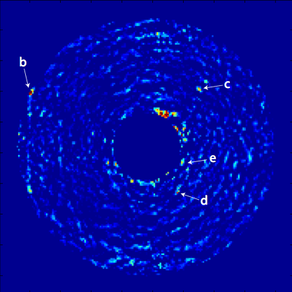
Radio telescope image of the galaxy 4C12.50, nearly 1.5 billion light-years from Earth. Inset shows detail of location at end of superfast jet of particles, where a massive gas cloud (yellow-orange) is being pushed by the jet.
(Credit: Morganti et al., NRAO/AUI/NSF)
It’s long been a mystery for astronomers: why aren’t galaxies bigger? What regulates their rates of star formation and keeps them from just becoming even more chock-full-of-stars than they already are? Now, using a worldwide network of radio telescopes, researchers have observed one of the processes that was on the short list of suspects: one supermassive black hole’s jets are plowing huge amounts of potential star-stuff clear out of its galaxy.
Astronomers have theorized that many galaxies should be more massive and have more stars than is actually the case. Scientists proposed two major mechanisms that would slow or halt the process of mass growth and star formation — violent stellar winds from bursts of star formation and pushback from the jets powered by the galaxy’s central, supermassive black hole.
“With the finely-detailed images provided by an intercontinental combination of radio telescopes, we have been able to see massive clumps of cold gas being pushed away from the galaxy’s center by the black-hole-powered jets,” said Raffaella Morganti, of the Netherlands Institute for Radio Astronomy and the University of Groningen.
The scientists studied a galaxy called 4C12.50, nearly 1.5 billion light-years from Earth. They chose this galaxy because it is at a stage where the black-hole “engine” that produces the jets is just turning on. As the black hole, a concentration of mass so dense that not even light can escape, pulls material toward it, the material forms a swirling disk surrounding the black hole. Processes in the disk tap the tremendous gravitational energy of the black hole to propel material outward from the poles of the disk.
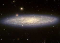
NGC 253, aka the Sculptor Galaxy, is also blowing out gas but as the result of star formation (Image: T.A. Rector/University of Alaska Anchorage, T. Abbott and NOAO/AURA/NSF)
At the ends of both jets, the researchers found clumps of hydrogen gas moving outward from the galaxy at 1,000 kilometers per second. One of the clouds has much as 16,000 times the mass of the Sun, while the other contains 140,000 times the mass of the Sun.
The larger cloud, the scientists said, is roughly 160 by 190 light-years in size.
“This is the most definitive evidence yet for an interaction between the swift-moving jet of such a galaxy and a dense interstellar gas cloud,” Morganti said. “We believe we are seeing in action the process by which an active, central engine can remove gas — the raw material for star formation — from a young galaxy,” she added.
The researchers published their findings in the September 6 issue of the journal Science.
I love it when scientists discover something unusual in nature. They have no idea what it is, and then over decades of research, evidence builds, and scientists grow to understand what’s going on.
My favorite example? Quasars.
Astronomers first knew they had a mystery on their hands in the 1960s when they turned the first radio telescopes to the sky.
They detected the radio waves streaming off the Sun, the Milky Way and a few stars, but they also turned up bizarre objects they couldn’t explain. These objects were small and incredibly bright.
They named them quasi-stellar-objects or “quasars”, and then began to argue about what might be causing them. The first was found to be moving away at more than a third the speed of light.
But was it really?
An artist’s conception of jets protruding from an AGN.Maybe we were seeing the distortion of gravity from a black hole, or could it be the white hole end of a wormhole. And If it was that fast, then it was really, really far… 4 billion light years away. And it generating as much energy as an entire galaxy with a hundred billion stars.
What could do this?
Here’s where Astronomers got creative. Maybe quasars weren’t really that bright, and it was our understanding of the size and expansion of the Universe that was wrong. Or maybe we were seeing the results of a civilization, who had harnessed all stars in their galaxy into some kind of energy source.
Then in the 1980s, astronomers started to agree on the active galaxy theory as the source of quasars. That, in fact, several different kinds of objects: quasars, blazars and radio galaxies were all the same thing, just seen from different angles. And that some mechanism was causing galaxies to blast out jets of radiation from their cores.
But what was that mechanism?
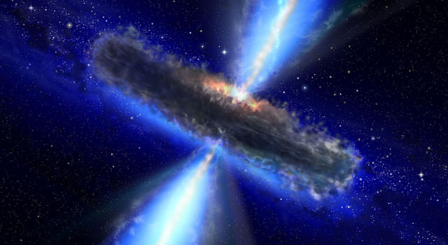
This artist’s concept illustrates a quasar, or feeding black hole, similar to APM 08279+5255, where astronomers discovered huge amounts of water vapor. Gas and dust likely form a torus around the central black hole, with clouds of charged gas above and below. Image credit: NASA/ESAWe now know that all galaxies have supermassive black holes at their centers; some billions of times the mass of the Sun. When material gets too close, it forms an accretion disk around the black hole. It heats up to millions of degrees, blasting out an enormous amount of radiation.
The magnetic environment around the black hole forms twin jets of material which flow out into space for millions of light-years. This is an AGN, an active galactic nucleus.
When the jets are perpendicular to our view, we see a radio galaxy. If they’re at an angle, we see a quasar. And when we’re staring right down the barrel of the jet, that’s a blazar. It’s the same object, seen from three different perspectives.
Supermassive black holes aren’t always feeding. If a black hole runs out of food, the jets run out of power and shut down. Right up until something else gets too close, and the whole system starts up again.
The Milky Way has a supermassive black hole at its center, and it’s all out of food. It doesn’t have an active galactic nucleus, and so, we don’t appear as a quasar to some distant galaxy.
We may have in the past, and may again in the future. In 10 billion years or so, when the Milky way collides with Andromeda, our supermassive black hole may roar to life as a quasar, consuming all this new material.
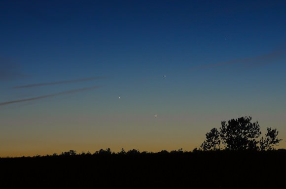
Planets conjunction over Mont-Saint-Michel, Normandy, France on May 26. Credit: Thierry Legault -
www.astrophoto.fr
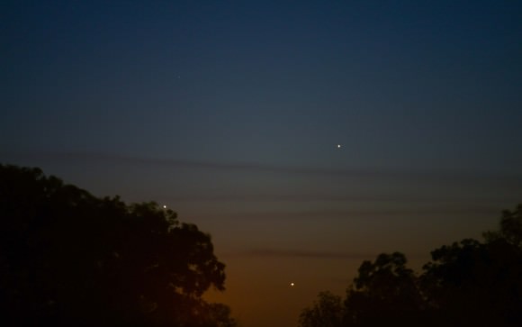
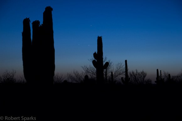
Triple planets (Venus/Jupiter/Mercury) conjunction over Mont-Saint-Michel, Normandy, France on May 26. Credit: Thierry Legault – www.astrophoto.fr Update: See expanded Conjunction astrophoto gallery below[/caption]
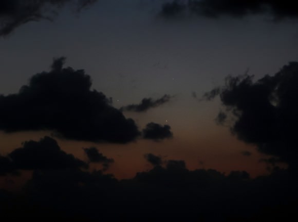
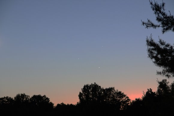
The rare astronomical coincidence of a spectacular triangular triple conjunction of 3 bright planets happening right now is certainly wowing the entire World of Earthlings! That is if our gallery of astrophotos assembled here is any indication.
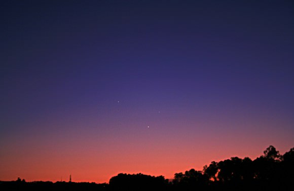
Right at sunset, our Solar System’s two brightest planets – Venus and Jupiter – as well as the sun’s closest planet Mercury are very closely aligned for about a week in late May 2013 – starting several days ago and continuing throughout this week.
And, for an extra special bonus – did you know that a pair of spacecraft from Earth are orbiting two of those planets?
Have you seen it yet ?
Well you’re are in for a celestial treat. The conjunction is visible to the naked eye – look West to Northwest shortly after sunset. No telescopes or binoculars needed.
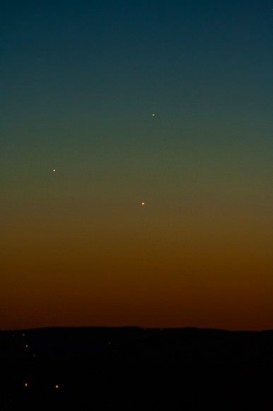
Triple conjunction shot on May 26 from a mile high in Payson,Az. 4 second exposure, ISO200, Canon 10D, 80mm f/5 lens. Credit: Chris Schur- http://www.schursastrophotography.com
Just check out our Universe Today collection of newly snapped astrophoto’s and videos sent to Nancy and Ken by stargazing enthusiasts from across the globe. See an earlier gallery – here.
Throughout May, the trio of wandering planets have been gradually gathering closer and closer.
On May 26 and 27, Venus, Jupiter and Mercury appear just 3 degrees apart as a spectacular triangularly shaped object in the sunset skies – which
adds a palatial pallet of splendid hues not possible at higher elevations.
And don’t dawdle if you want to see this celestial feast. The best times are 30 to 60 minutes after sunset – because thereafter they’ll disappear below the horizon.
The sky show will continue into late May as the planets alignment changes every day.
On May 28, Venus and Jupiter close in to within just 1 degree.
And on May 30 & 31, Venus, Jupiter and Mercury will form an imaginary line in the sky.
Triple planetary conjunctions are a rather rare occurrence. The last one took place in May 2011. And we won’t see another one until October 2015.
Indeed the wandering trio are also currently the three brightest planets visible. Venus is about magnitude minus 4, Jupiter is about minus 2.
While you’re enjoying the fantastic view, ponder this: The three planets are also joined by two orbiting spacecraft from humanity. NASA’s MESSENGER is orbiting Mercury. ESA’s Venus Express is orbiting Venus. And NASA’s Juno spacecraft is on a long looping trajectory to Jupiter.
Send Ken you conjunction photos to post here.
And don’t forget to “Send Your Name to Mars” aboard NASA’s MAVEN orbiter- details here. Deadline: July 1, 2013
…………….
Learn more about Conjunctions, Mars, Curiosity, Opportunity, MAVEN, LADEE and NASA missions at Ken’s upcoming lecture presentations:
June 4: “Send your Name to Mars” and “CIBER Astro Sat, LADEE Lunar & Antares Rocket Launches from Virginia”; Rodeway Inn, Chincoteague, VA, 8:30 PM
June 11: “Send your Name to Mars” and “LADEE Lunar & Antares Rocket Launches from Virginia”; NJ State Museum Planetarium and Amateur Astronomers Association of Princeton (AAAP), Trenton, NJ, 730 PM.
May 25 conjunction over Malta. Canon 450D with a 55mm. lens and an exposure of 1/2 second at ISO 200 on a tripod. Credit: Leonard Ellul-MercerMay 26 triple conjunction from Warwick, NY snapped from Canon Rebel, 100mm – 300mm lens. Credit: Pietro CarboniTriple conjunction from Hondo, Texas taken with a Nikon D800 @ ISO 400 and a 2 second exposure with a Nikon 300mm Lens at F/4. Credit: Adrian New Sunset conjunction with fast moving clouds on May 26 through 10 x 50 binoculars from a seashore town -Marina di Pisa, Tuscany, Italy. Credit: Giuseppe Petricca
Caption: Taken on 2013-05-23 from Salem, Missouri. Canon T1i, Nikkor 105mm lens. 297 1/4s at 1s interval. Images assembled by QuickTime Pro. Credit: Joseph Shuster
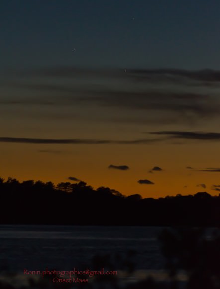
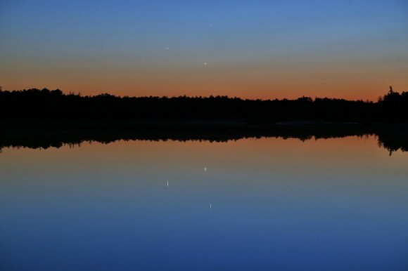
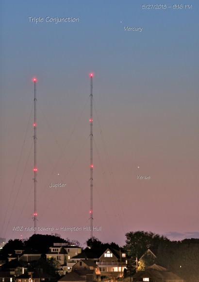
May 26 sunset conjunction from Princeton, NJ. Credit: Ken Kremer -kenkremer.comTriple Planetary conjunction over Onset MA. Shot with a Nikon d7000 1/200 f 4 iso 100 at 110mm. Credit: Phillip DamianoPanoramic view over Almada City and Lisbon at the Nautical Twilight, with the Full moon rising above the Eastern horizon (right side of the image), while at the same time but in the opposite direction, the planets Venus, Mercury and Jupiter, are aligned in a triangle formation, setting in the Western horizon (left side of the image).In this panoramic picture is also visible the smooth light transition in the sky, with the end of Nautical Twilight and the beginning of Astronomical Twilight (almost night), at right. Facing to North, is visible the great lighted Monument Christ the King and at the left side of it, part of the 25 April Bridge that connects Almada to Lisbon. Canon 50D – ISO200; f/4; Exp. 1,6 Sec; 35mm. Panoramic of 10 images with about 200º, taken at 21h42 in 25/05/2013. Credit: Miguel Claro – www.miguelclaro.comThe triple conjunction of Venus, Mercury and Jupiter as seen over an Arizona desert landscape. Credit and copyright: Robert Sparks.Jupiter, Venus and Mercury triple conjunction seen here reflecting off Chatsworth Lake in Chatsworth, NJ. Jupiter (on the left) was 2.4° from Mercury (upper-right in the sky) and 2.0° from Venus (bottom right in the sky), while Venus and Mercury were 1.9° apart. Venus was at 2.6° altitude. Canon EOS 6D, 105 mm focal length, 1.3 seconds, f/6.3, ISO 800. Credit: Joe Stieber – sjastro.org/Triple conjunction on May 27 with WBZ radio towers south east of Boston. Hampton Hill, Hull, MA. Nikon D3x -iso200- 1.3 sec.at f2.8. Credit: Richard W. Green
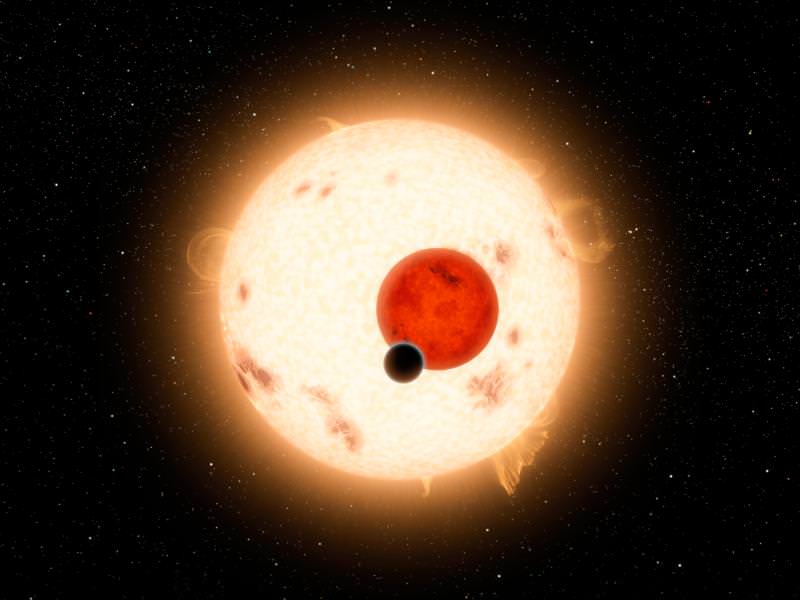
Kepler-16b is but one example of an uncanny world. It orbits two suns. Credit: Discovery
Exoplanets are uncanny. Some seem to have walked directly out of the best science-fiction movies. For example, we’ve discovered a planet consisting purely of water (GJ 1214b) and one with two suns (Kepler 16b). Some planets nearly scrape their host stars once every orbit, while others exist in darkness without a host star at all. The field of exoplanet research is moving beyond detecting exoplanets to characterizing them – understanding which molecules are present and if they might possibly harbor life.
A key research element in characterizing these alien worlds is observing their atmospheres. But how exactly do astronomers do this? We can’t simply tug the planet toward us to get a closer look. It’s also incredibly difficult to directly image their atmospheres from afar. Why? Stars are incredibly bright in comparison to their puny, barely reflective, and nearby exoplanets. So a direct image of an exoplanet’s atmosphere seemed out of the question – until recently.
It may be tricky to directly image an exoplanet’s atmosphere, but astronomers always have quite a few tricks up their sleeves. The first one is in mounting an instrument called a coronagraph on your telescope. This instrument blocks out the star’s light, leaving an image of the exoplanet alone. Another trick, known as adaptive optics, is to send a laser beam through the atmosphere. The changes in the laser allow us to monitor changes in the atmosphere, providing corrections to clean and smooth the image.
HR 8799, a large star orbited by four known giant planets, is relatively nearby (remember that ‘nearby’ is an astronomers way of saying that it is still pretty far, or in this case 130 light years away). In 2008, three of the planets were directly imaged using the Gemini and Keck telescopes on Mauna Kea, Hawaii. In 2010, the fourth planet, which was closest to the star and therefore the most difficult to see was directly imaged by the Keck telescope.
Direct image of the HR 8799 system. The star has been blocked and all four planets can clearby be seen. Credit: Oppenheimer et al. 2013
A direct image of an exoplanet’s atmosphere may tell us what color the atmosphere appears to be, and how thick the atmosphere is, but it gives us little more information. We need to know the atmospheric composition – the specific molecules and their abundances that are present within the atmosphere itself. If we’re looking at the question of habitability we need to know if there is water in the atmosphere or maybe carbon dioxide.
The key is in mounting a spectrograph on the telescope. Instead of collecting the overall light from the planet, that light is broken up into a spectrum of wavelengths. Imagine seeing a rainbow after a thunderstorm. That rainbow is simply the light from the sun broken up across all visible wavelengths due to ice crystals in our atmosphere. Molecules emit light at specific wavelengths, leaving well-known fingerprints that may be identified in a lab on Earth, in a rainbow in the sky, or in the spectrum of an exoplanet located 130 light years away.
When astronomers mounted their instrumentation (i.e. a coronagraph, an adaptive optics system, and a spectrograph) known as Project 1640 onboard the Palomar 5m Hale Telescope, they were able to shed new light on the HR 7899 system. Only last month one of its exoplanets revealed a mixture of water vapor and carbon monoxide in its atmosphere, but the story has changed. See a previous article in Universe Today.
Project 1640 observed not one – but four atmospheres at once. Gautam Vasisht of JPL explains, “in just one hour, we were able to get precise composition information about four planets around one overwhelmingly bright star.” These four exoplanets are believed to be coeval, in that they formed from a protoplanetary disk at roughly the same time. They also have the same luminosity and temperature, leading to the assumption that they are roughly similar to each other. But results show that they all have radically different spectra, and therefore different chemical compositions!
More specifically, HR 8799 b and d contain carbon dioxide, b and c contain ammonia, d and e contain methane, and b, d, and e contain acetylene. Noticing a few trends? There really aren’t any! Not only are these planets different from each other, they are also different from any other known objects. Acetylene, for example, has never been convincingly identified in a sub-stellar object outside the solar system. While the varying spectra pose many questions, one thing is clear: the diversity of planets must be greater than previously thought!
This is only the first exoplanet system for which we’ve obtained direct spectra of all exoplanet atmospheres. Project 1640 will conduct a 3-year survey of 200 nearby stars. The hope is to find hot Jupiters located far from their host star. While this is what the current technique allows astronomers to detect, it will also teach astronomers how Earth-like planets form.
“The outer giant planets dictate the fate of rocky ones like Earth. Giant planets can migrate in toward a star, and in the process, tug the smaller, rocky planets around or even kick them out of the system. We’re looking at hot Jupiters before they migrate in, and hope to understand more about how and when they might influence the destiny of the rocky, inner planets,” explained Vasisht.
In an attempt to understand our own blue marble, astronomers point their telescopes at uncanny worlds light years away. Project 1640 will block the light of distant stars in order to shed light on distant worlds as well as our own.
When it comes to immediate and widespread appeal, astronomical diagrams have it tough. There’s a reason we have Most Awesome Space Images of 2012, but not “Astronomy’s coolest diagrams 2012.” But arguably, diagrams (more concretely: plots that help us visualize one or more physical quantities) are the key to understanding what’s up with all those objects whose colorful images we know and love.
To be sure, some diagrams have become quite famous. Take the Hubble diagram plotting galaxies’ redshifts against their distances: Its earliest version marks the discovery that we live in an expanding universe. A more recent incarnation, which shows how cosmic expansion is accelerating, won its creators the 2011 Nobel prize in physics.
Another famous diagram is the Hertzsprung-Russell diagram (HR diagram, for short, shown above.) A single star doesn’t tell you all that much about stars in general. But if you plot the brightnesses and colors of many stars, patterns begin to emerge – such as the distinctive broad band of the “main sequence” bisecting the HR diagram diagonally, the realm of the giants and supergiants to its upper right and the White Dwarfs below on the left.
When astronomers first recognized those patterns, they took the first steps towards our modern understanding of how stars evolve over time.
The first HR diagram was published by the US astronomer Henry Norris Russell in 1913 (or at least described in words, if you look at the article); Hubble’s first diagram in 1929. Off the top of my head, I cannot think of any famous astronomical plot with more recent roots.
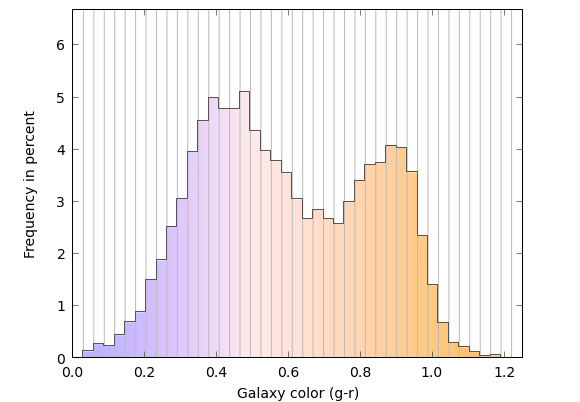
But that doesn’t mean there aren’t some plots that by rights should be famous. Here’s my rendition of what, back in 2003, must have been one of the first comprehensive examples of its kind (from this article by Blanton et al. 2003). The diagram shows the colors of many different galaxies, and how frequently or less frequently one encounters galaxies with those particular colors:
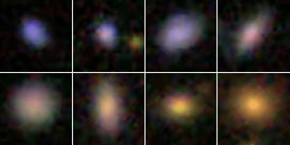
If you’re not familiar with this type of plot, it’s best to think of the vertical lines as dividing the diagram into bins – think “glass cylinders you can put stuff in.” Next, obtain a sample of images of distant galaxies. Here are some that I retrieved with the Skyserver Tool kindly provided by the folks who produced the Sloan Digital Sky Survey (SDSS) — a huge survey that, in its latest data release, lists more than 1.4 million galaxies:
Galaxies from the Sloan Digital Sky Survey.
If these images are less detailed than what you’re used to, it’s because the galaxies are very far away even by extragalactic standards — their light takes almost 1.3 billion years to reach us. Even so, you can readily distinguish the galaxies’ different colors.
With that information, back to our (glass) bins. Think of the differently colored galaxies as differently colored marbles. Each bin accepts galaxies of one particular shade of color – so put each marble into the appropriate bin! As you do, some of the bins will fill up more, some less. The colored bars indicate each bin’s filling level. On the scale to the left, you can read off the corresponding numbers. For instance, the best-filled bin contains a little more than 5 percent of all the galaxy-marbles.
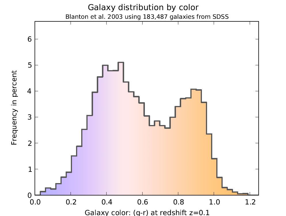
Now that you know how to read the diagram, let’s remove the extra vertical lines. In a paper published in an astronomical research journal, this is what a “histogram” of this kind would look like:
Galaxy distribution by color. Credit: Markus Pössel
I’ve left the coloring in even though you’d probably not find it in an astronomical paper. The astronomers’ own measure of color, denoted “g-r” on the horizontal axis, is a bit technical — let’s ignore those details and stick with the colors we see in the diagram.
To fill the bins in this particular diagram, the astronomers from the SDSS collaboration sorted 183,487 galaxies from their survey by color.
So what does the diagram tell us? Evidently, there are two peaks: one near the bluish end on the left, one near the reddish end on the right. That indicates two distinct types of galaxies. Galaxies of the first kind are, on average, of a bluish-white color, with some specimens a little more and some a little less blue (which is why the peak is a little broad). Galaxies of the other kind are, on average, much redder.
A galaxy’s color derives from its stars. A bluish galaxy is one with bluish stars. Bluish stars are hotter than reddish ones. (Think of heating metal: It starts out a dull red, becomes orange, then white-hot; if you could make metal even hotter, it would radiate bluish.) Hot stars are more massive than cooler stars, and they live fast and die young — the most massive ones die after much less than a million years, a fleeting moment compared with our Sun’s estimated lifetime of ten billion years. For a galaxy to glow an overall blue, it must have a steady supply of these short-lived bluish stars, producing new blue stars in sufficient quantities as the old ones burn out. So evidently, the galaxies of the bluish kind are continually producing new bluish stars. Since there is no known mechanism that makes a galaxy produce only bluish stars, we can drop the qualifier: these galaxies are continually producing new stars.
The reddish galaxies, on the other hand, produce hardly any new stars. If they did, then by all we know about star formation there should be sufficient bluish stars around to give these galaxies an overall bluish tint. Without any new stars, all that is left are long-lived, less massive stars, and those tend to be cooler and more reddish.
The existence of two distinct classes of galaxies — star-forming vs. “red and dead” — is a driving force behind current research on galaxy evolution in much the same way the HR diagram was for stellar evolution. Why are there two distinct kinds? What makes the bluish galaxies produce stars, and what prevents the reddish ones? Do galaxies move from one camp to the other over time? And if yes, how and in which direction? When you read an article like this about the care and feeding of teenage galaxies, or this one about galaxies recycling their gas, it’s all about astronomers trying to find pieces of the puzzle of why there are these two populations.
This diagram clearly deserves wider public recognition. And no doubt there are many other, equally under-appreciated astronomical plots. Please help me give them some of the recognition they deserve: Which diagrams have done the most to increase your understanding of what’s out there? Which have surprised you? Which have sent a thrill down your spine? Please post a link or a description, and let’s see if we can create a “Top 10” list of astronomical diagrams. And who knows: We might even try for an “Astronomy’s coolest diagrams 2013” at the end of the year.
__________________________________________
Additional information about how the two-peak galaxy diagram was made, including different versions for download and the python script that produced it, can be found here. If you do want to know about the technical details about the color: The values on the x axis correspond to g-r, where g is the star’s brightness (expressed in the usual astronomical magnitude system) through one particular greenish filter and r the brightness through one particular reddish filter. Details about the ugriz filter system used can be found on this SDSS page. And in case you’re worrying about the effect cosmic redshift might have had on the galaxies in the sample: the astronomers took care to compensate for that particular effect, correcting the colors to appear as they would if each of the galaxies were so far away that its light would take 1.29 billion years to reach us (that is, at a cosmic redshift of z=0.1).
Many thanks to Kate H.R. Rubin for pointing me to the galaxy diagram and for helpful discussions.
Online Messier Marathon with the Virtual Telescope Project.
Have you ever done a Messier Marathon? Want to try it online from the comfort of your own home? Astrophysicist Gianluca Masi will host a webcast today (April 9, 2013) at 18:00 UTC (2 pm EDT) (update: this webcast has been postponed due to clouds. We’ll post the new date and time when it becomes available). You can join in at this link, and explore the many treasures of the famous Messier Catalog. Masi said they will try to see as many of 110 objects in the Messier Catalog as possible in a single viewing session. This is what is called a Messier Marathon!
This is the fifth time the Virutal Telescope Project has attempted this, and they’ve had great success previously. Masi is doing the Marathon their robotic telescopes, and will provide real time images and live comments, along with answering your questions and “sharing your passion and excitement with friends from all around the world.”
Want to learn more about our Universe or refresh your astronomical knowledge? Cosmoquest has two new online astronomy classes, and they are a great opportunity expand your horizons! The two classes are “The Sun and Stellar Evolution” (April 15 – May 8, 2013) and “Introduction to Cosmology” (April 23 – May 16, 2013) Cosmoquest offers the convenience of an online class along with live (and lively!) interaction with your instructor and a small group astronomy enthusiasts like yourself. The lectures are held in Google+ Hangouts, with course assignments and homework assigned via Moodle.
The instructors are likely well-known to UT readers. Research assistant and blogger Ray Sanders (Dear Astronomer and UT) will be teaching the stellar evolution class and astronomer and writer Dr. Matthew Francis will be leading the cosmology course.
The cost for the class is $240, and the class is limited to 8 participants, with the possibility for an additional 5 participants. Both instructors say no prior knowledge of cosmology or astronomy is needed. There will be a little math, but it will be on the high school algebra level. Concepts will be heavily emphasized.
The Sun is a fascinating topic of study, which allows solar astronomers to better understand the physical processes in other stars. During this 4-week / 8-session course, we’ll explore the Sun and Solar Evolution from an astronomer’s point of view. Our course
will begin with an overview of the Sun, and solar phenomenon. We’ll also explore how stars are formed, their lifecycles, and the
incredible events that occur when stars reach the end of their lives. The course will culminate with students doing a short presentation on a topic related to the Sun or Stellar Evolution.
Cosmology is the study of the structure, contents, and evolution of the Universe as a whole. But what do cosmologists really study? In this 8-session course, we’ll look at cosmology from an astronomy point of view: taking what seems like too big of a subject and showing how we can indeed study the Universe scientifically. The starting point is the smallest chunk of the Universe that is representative of everything we can see: the Cosmic Box.
Class level: No prior knowledge of cosmology or astronomy is needed. There will be a little math, but it will be on the high school algebra level: the manipulation of ratios and use of some important equations. The emphasis is on concepts!
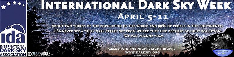
International Dark Sky Week banner, courtesy Sean Parker Photography.
Take the next few nights to celebrate the stars! The International Dark Sky Week is a worldwide event, and part of Global Astronomy Month – going on now! The goals of IDSW are to appreciate the beauty of the night sky and to raise awareness of how poor-quality lighting creates light pollution.
The International Dark-Sky Association says that light pollution is a growing problem: “Not only does it have detrimental effects on our views of the night sky, but it also disrupts the natural environment, wastes energy, and has the potential to cause health problems.”
Here are some ways that the IDA suggests how you can spread the word about IDSW during April 5-11 — as well and all year long:
Join IDA online! Post about dark skies awareness on the social media sites, and you can follow the IDA on Facebook, Twitter, G+ and any other social media you like. And if you would like to become a partner email [email protected] to learn more. See a list of existing partners here.
Check around your home. Make sure your outdoor-lighting fixtures are well shielded — or at least angled down — to minimize “light trespass” beyond your property. Do you have security lights that stay on all night? Consider adding a motion-detector, which can pay for itself in energy savings in just a few months. You’ll find lots of great suggestions in “Good Neighbor Outdoor Lighting” and you can perform your own outdoor lighting audit.
Talk to your neighbors. Explain that bright, glaring lights are actually counterproductive to good nighttime vision. Glare diminishes your ability to see well at night, because the pupils of your eyes constrict in response to the glare — even though everything else around you is dark. Show them this handout.
International Dark Sky Week poster. Image courtesy Sean Parker Photography.
Ask your local library if you can put up an IDA poster showing good and bad lights. Include a photo of the Earth at night, and take some pictures around town that show examples of good and bad lighting.
Become a Citizen Scientist with GLOBE at Night and similar programs, observe light pollution wherever you are and contribute to reports coming in from across the globe about light pollution. Or join GLOBE at Night’s Adopt-A-Street program and ‘map’ light pollution in your community.
Become a Dark Sky Ranger. Teachers and families can do these activities that include an outdoor lighting audit, a game, and hands-on crafts to help visualize the night sky better. In English.In Portuguese.
Attend or throw a star party! International Dark Sky Week is a great opportunity to dust off the old telescope in your attic and use it share in the wonder of the universe with your family, friends, and neighbors. Visit the Night Sky Network to find a calendar of star parties or to find an astronomy club in your area. Click here to find out what’s up in the sky. This activity book is full of great activities for budding stargazers of all ages!
“No scientific discovery is named after its discoverer,” – Stigler/Merton.
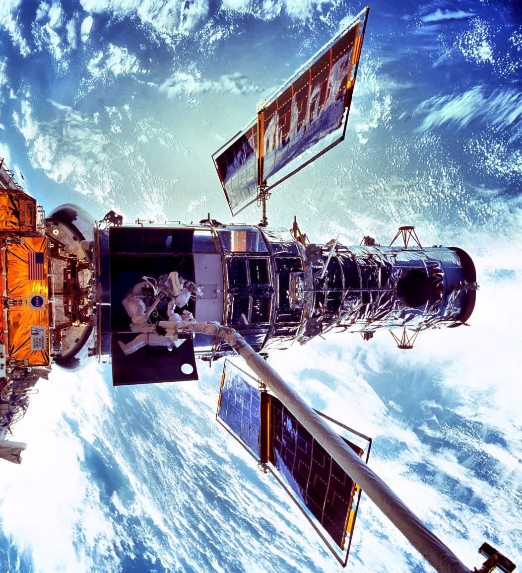
Edwin Hubble’s contributions to astronomy earned him the honor of having his name bestowed upon arguably the most famous space telescope (the Hubble Space Telescope, HST). Contributions that are often attributed to him include the discovery of the extragalactic scale (there exist countless other galaxies beyond the Milky Way), the expanding Universe (the Hubble constant), and a galaxy classification system (the Hubble Tuning Fork). However, certain astronomers are questioning Hubble’s pre-eminence in those topics, and if all the credit is warranted.
“[The above mentioned] discoveries … are well-known … and most astronomers would associate them solely with Edwin Hubble; yet this is a gross oversimplification. Astronomers and historians are beginning to revise that standard story and bring a more nuanced version to the public’s attention,” said NASA scientist Michael J. Way, who just published a new study entitled “Dismantling Hubble’s Legacy?”
Has history clouded our view of Hubble the man? Or are his contributions seminal to where we are today in astronomy?
Assigning credit for a discovery is not always straightforward, and Way 2013 notes, “How credit is awarded for a discovery is often a complex issue and should not be oversimplified – yet this happens time and again. Another well-known example in this field is the discovery of the Cosmic Microwave Background.” Indeed, controversy surrounds the discovery of the Universe’s accelerated expansion, which merely occurred in the late 1990s. Conversely, the discoveries attributed to Hubble transpired during the ~1920s.
The Hubble Space Telescope (image credit: NASA, tweaked by D. Majaess).
Prior to commencing this discussion, it’s emphasized that Hubble cannot defend his contribution since he died long ago (1889-1953). Moreover, we can certainly highlight the efforts of other individuals whose seminal contributions were overlooked without mitigating Hubble’s pertinence. The first topic discussed here is the discovery of the extragalactic scale. Prior to the 1920s it was unclear whether the Milky Way galaxy and the Universe were synonymous. In other words, was the Milky Way merely one among countless other galaxies?
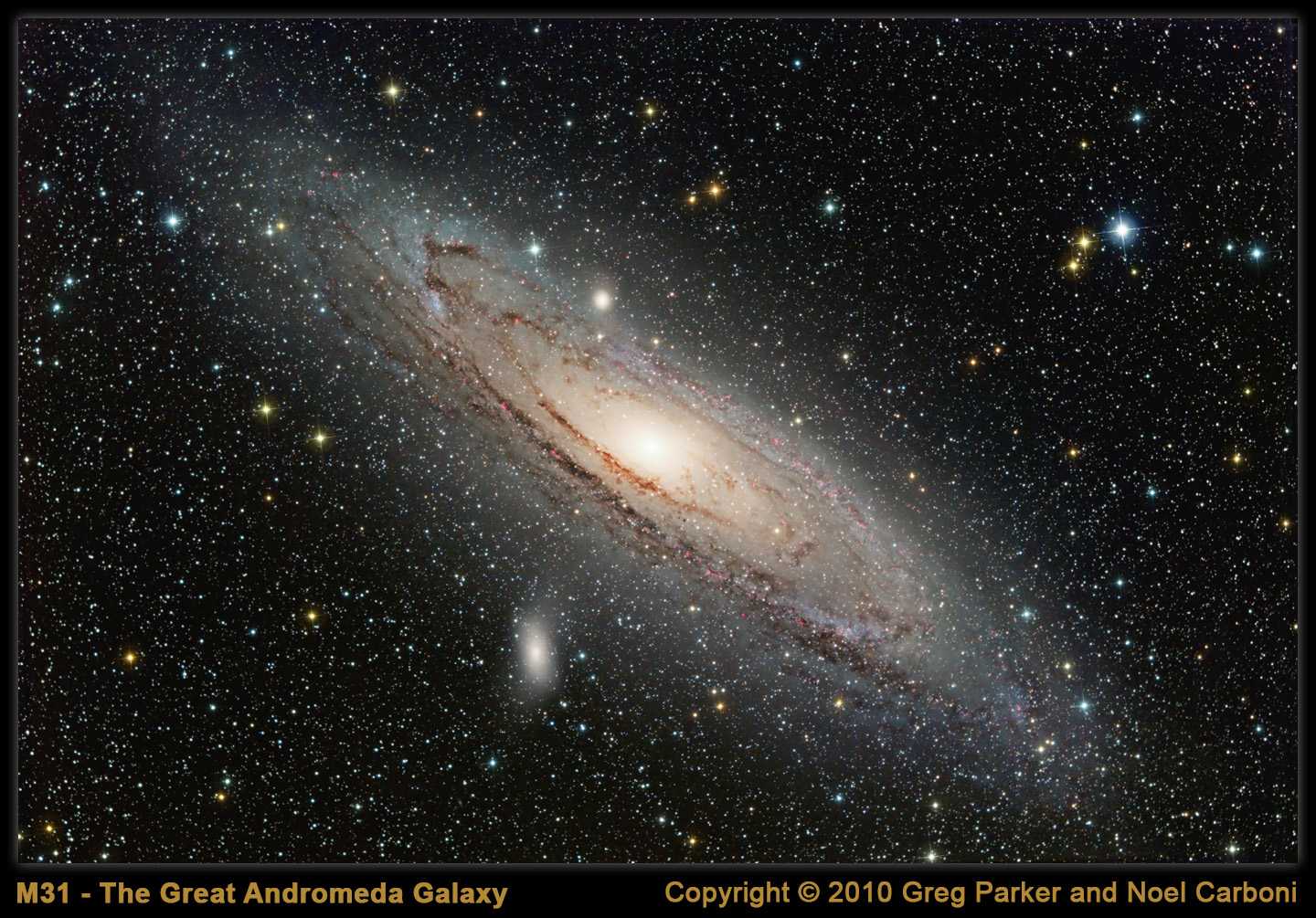
Astronomers H. Shapley and H. Curtis argued the topic in the famed Island Universe debate (1920). Curtis believed in the extragalactic Universe, whereas Shapley took the opposing view (see also Trimble 1995 for a review). In the present author’s opinion, Hubble’s contributions helped end that debate a few years later and changed the course of astronomy, namely since he provided evidence of an extragalactic Universe using a distance indicator that was acknowledged as being reliable. Hubble used stars called Cepheid variables to help ascertain that M31 and NGC 6822 were more distant than the estimated size of the Milky Way, which in concert with their deduced size, implied they were galaxies. Incidentally, Hubble’s distances, and those of others, were not as reliable as believed (e.g., Fernie 1969, Peacock 2013). Peacock 2013 provides an interesting comparison between distance estimates cited by Hubble and Lundmark with present values, which reveals that both authors published distances that were flawed in some manner. Having said that, present-day estimates are themselves debated.
Hubble’s evidence helped convince even certain staunch opponents of the extragalactic interpretation such as Shapley, who upon receiving news from Hubble concerning his new findings remarked (1924), “Here is the letter that has destroyed my universe.” Way 2013 likewise notes that, “The issue [concerning the extragalactic scale] was effectively settled by two papers from Hubble in 1925 in which he derived distances from Cepheid variables found in M31 and M33 (Hubble 1925a) of 930,000 light years and in NGC 6822 (Hubble 1925c) of 700,000 light years.”
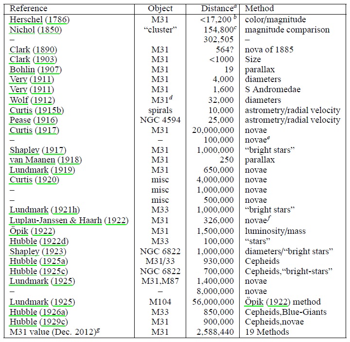
However, as table 1 from Way 2013 indicates (shown below), there were numerous astronomers who published distances that implied there were galaxies beyond the Milky Way. Astronomer Ian Steer, who helps maintain the NASA/IPAC Extragalactic Database of Redshift-Independent Distances (NED-D), has also compiled a list of 290 distances to galaxies published before 1930. Way 2013 added that, “Many important contributions to this story have been forgotten and most textbooks in astronomy today, if they discuss the “Island Universe” confirmation at all, bestow 100% of the credit on Hubble with scant attention to the earlier observations that clearly supported his measurements.”
Thus Hubble did not discover the extragalactic scale, but his work helped convince a broad array of astronomers of the Universe’s enormity. However, by comparison to present-day estimates, Hubble’s distances are too short owing partly to the existing Cepheid calibration he utilized (Fernie 1969, Peacock 2013 also notes that Hubble’s distances were flawed for other reasons). That offset permeated into certain determinations of the expansion rate of the Universe (the Hubble constant), making the estimate nearly an order of magnitude too large, and the implied age for the Universe too small.
Way 2013 notes, “Table 1 lists all of the main distance estimates to spiral nebulae (known to this author) from the late 1800s until 1930 when standard candles began to be found in spiral nebulae [galaxies].” (image credit: Way 2013/arXiv).Hubble’s accreditation as the discoverer of the expanding Universe (the Hubble constant) has generated considerable discussion, which is ultimately tied to the discovery of a relationship between a galaxy’s velocity and its distance. An accusation even surfaced that Hubble may have censored the publication of another scientist to retain his pre-eminence. That accusation has since been refuted, but provides the reader an indication of the tone of the debate (see Livio 2012 (Nature), and references therein).
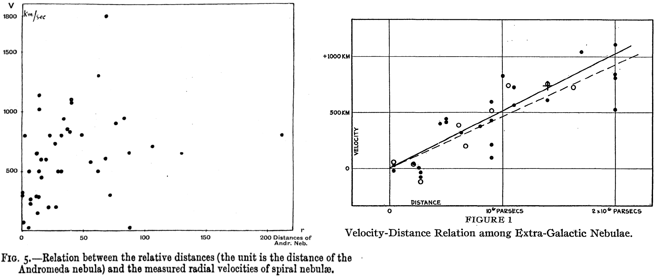
Hubble published his findings on the velocity-distance relation in 1929, under the unambiguous title, “A Relation Between Distance and Radial Velocity Among Extra-Galactic Nebulae”. Hubble 1929 states at the outset that other investigations have sought, “a correlation between apparent radial velocities and distances, but so far the results have not been convincing.” The key word being convincing, clearly a subjective term, but which Hubble believes is the principal impetus behind his new effort. In Lundmark 1924, where a velocity versus distance diagram is plotted for galaxies (see below), that author remarks that, “Plotting the radial velocities against these relative distances, we find that there may be a relation between the two quantities, although not a very definite one.” However, Hubble 1929 also makes reference to a study by Lundmark 1925, where Lundmark underscores that, “A rather definite correlation is shown between apparent dimensions and radial velocity, in the sense that the smaller and presumably more distant spirals have the higher space velocity.”
Hubble 1929 provides a velocity-distance diagram (featured below) and also notes that, “the data indicate a linear correlation between distances and velocities”. However, Hubble 1929 explicitly cautioned that, “New data to be expected in the near future may modify the significance of the present investigation, or, if confirmatory, will lead to a solution having many times the weight. For this reason it is thought premature to discuss in detail the obvious consequences of the present results … the linear relation found in the present discussion is a first approximation representing a restricted range in distance.” Hubble implied that additional effort was required to acquire observational data and place the relation on firm (convincing) footing, which would appear in Hubble and Humason 1931. Perhaps that may partly explain, in concert with the natural tendency of most humans to desire recognition and fame, why Hubble subsequently tried to retain credit for the establishment of the velocity-distance relation.
Hubble 1929 conveyed that he was aware of prior (but unconvincing to him) investigations on the topic of the velocity-distance relation. That is further confirmed by van den Bergh 2011, who cites the following pertinent quote recounted by Hubble’s assistant (Humason) for an oral history project, “The velocity-distance relationship started after one of the IAU meetings, I think it was in Holland [1928]. And Dr. Hubble came home rather excited about the fact that two or three scientists over there, astronomers, had suggested that the fainter the nebulae were, the more distant they were and the larger the red shifts would be. And he talked to me and asked if I would try and check that out.”
The velocities of galaxies plotted as a function of their distance, from Lundmark 1924 (left) and Hubble 1929 (right). Note the separate scales on the x-axis. Peacock 2013 demonstrates that distances cited by both authors were ultimately flawed, and problems (albeit less acute) likewise exist with modern distances (image credit: Lundmark/MNRAS/Hubble/PNAS, assembled by D. Majaess).
Hubble 1929 elaborated that, “The outstanding feature, however, is the possibility that the velocity-distance relation may represent the de Sitter effect, and hence that numerical data may be introduced into discussions of the general curvature of space.” de Sitter had proposed a model for the Universe whereby light is redshifted as it travels further from the emitting source. Hubble suspected that perhaps his findings may represent the de Sitter effect, however, Way 2013 notes that, “Thus far historians have unearthed no evidence that Hubble was searching for the clues to an expanding universe when he published his 1929 paper (Hubble 1929b).” Indeed, nearly two decades after the 1929 publication, Hubble 1947 remarks that better data may indicate that, “redshifts may not be due to an expanding universe, and much of the current speculation on the structure of the universe may require re-examination.” It is thus somewhat of a paradox that, in tandem with the other reasons outlined, Hubble is credited with discovering that the Universe is expanding.
The term redshift stems from the fact that when astronomers (e.g., V. Slipher) examined the spectra of certain galaxies, they noticed that although a particular spectral line should have appeared in the blue region of the spectrum (as measured in a laboratory): the line was actually shifted redward. Hubble 1947 explained that, “light-waves from distant nebulae [galaxies] seem to grow longer in proportion to the distance they have travelled It is as though the stations on your radio dial were all shifted toward the longer wavelengths in proportion to the distances of the stations. In the nebular [galaxy] spectra the stations (or lines) are shifted toward the red, and these redshifts vary directly with distance–an approximately linear relation. This interpretation lends itself directly to theories of an expanding universe. The interpretation is not universally accepted, but even the most cautious of us admit that redshifts are evidence either of an expanding universe or of some hitherto unknown principle of nature.”
Top, spectra for galaxies that are redshifted (image credit: JPL/Caltech/Planck).
As noted above, Hubble was not the first to deduce a velocity-distance relation for galaxies, and Way 2013 notes that, “Lundmark (1924b): first distance vs. velocity plot for spiral nebulae [galaxies] …Georges Lemaitre (1927): derived a non–static solution to Einstein’s equations and coupled it to observations to reveal a linear distance vs. redshift relation with a slope of 670 or 575 km/s/Mpc (depending on how the data is grouped) …” Although Hubble was aware of Lundmark’s research, he and numerous other astronomers were likely unaware of the now famous 1927 Lemaitre study, which was published in an obscure journal (see Livio 2012 (Nature), and discussion therein). Steer 2013 notes that, “Lundmark’s [1924] distance estimates were consistent with a Hubble constant of 75 km/s/Mpc [which is close to recent estimates].” (see also the interpretation of Peacock 2013). Certain distances established by Lundmark appear close to present determinations (e.g., M31, see the table above).
So why was Hubble credited with discovering the expanding Universe? Way 2013 suggests that, “Hubble’s success in gaining credit for his … linear distance-velocity relation may be related to his verification of the Island Universe hypothesis –after the latter, his prominence as a major player in astronomy was affirmed. As pointed out by Merton (1968) credit for simultaneous (or nearly so) discoveries is usually given to eminent scientists over lesser-known ones.” Steer told Universe Today that, “Lundmark in his own words did not find a definite relation between redshift and distance, and there is no linear relation overplotted in his redshift-distance graph. Where Lundmark used a single unproven distance indicator (galaxy diameters), cross-checked by a single unproven distance to the Andromeda galaxy, Hubble used multiple indicators including one still in use (brightest stars), cross-checked with distances to multiple galaxies based on Cepheids variables stars.”
Concerning assigning credit for the discovery of the expansion of the Universe, Way 2013 concludes that, “Overall we find that Lemaitre was the first to seek and find a linear relation between distance and velocity in the context of an expanding universe, but that a number of other actors (e.g. Carl Wirtz, Ludwik Silberstein, Knut Lundmark, Edwin Hubble, Willem de Sitter) were looking for a relation that fit into the context of de Sitter’s [Universe] Model B world with its spurious radial velocities [the redshift].” A partial list of the various contributors highlighted by van den Bergh 2011 is provided below.
“The history of the discovery of the expansion of the Universe may be summarized [above],” van den Bergh 2011 (image credit: van den Bergh/JRASC/arXiv).Way and Nussbaumer 2011 assert that, “It is still widely held that in 1929 Edwin Hubble discovered the expanding Universe … that is incorrect. There is little excuse for this, since there exists sufficient well-supported evidence about the circumstances of the discovery.”
In sum, the author’s personal opinion is that Hubble’s contributions to astronomy were seminal. Hubble helped convince astronomers of the extragalactic distance scale and that a relationship existed between the distance to a galaxy and its velocity, thus propelling the field and science forward. His extragalactic distances, albeit flawed, were also used to draw important conclusions (e.g., by Lemaitre 1927). However, it is likewise clear that other individuals are meritorious and deserve significant praise. The contributions of those scientists should be highlighted in parallel to Hubble’s research, and astronomy textbooks should be revised to emphasize those achievements A fuller account should be cited of the admirable achievements made by numerous astronomers working in synergy during the 1920s.
There are a diverse set of opinions on the topics discussed, and the reader should remain skeptical (of the present article and other interpretations), particularly since knowledge of the topic is evolving and more is yet to emerge. Two talks from the “Origins of the Expanding Universe: 1912-1932” conference are posted below (by H. Nussbaumer and M. Way), in addition to a talk by I. Steer from a separate event.
Here’s a quick overview from Jane Houston Jones from JPL of what you can see in the night skies during April 2013. Of special interest is that Saturn’s north pole is now tilted towards Earth, giving us the best view of the rings since 2006.


!["The history of the discovery of the expansion of the Universe may be summarized [above]", S. van den Bergh 2011. Image credit: S. van den Bergh/JRASC/arXiv.](https://www.universetoday.com/wp-content/uploads/2013/04/history.jpg)