Universe Today Guide to the Messier Objects


Well, Tammy’s done it again. Remember the Universe Today Guide to the Constellations? Well now Tammy has completed another monster volume. The Universe Today Guide to the Messier Objects. This is a guide to all 110 Messier Objects, from M1 (the Crab Nebula) to M110 (a satellite galaxy to Andromeda), and everything in between.

In addition to descriptions of the individual Messier Objects, there’s also a nice introduction to the Messier Objects, a guide to doing a Messier marathon, and suggestions for stretching your Messier marathon out to a week.

If you’ve got any questions, comments or feedback, please let us know. I’m sure there are going to be some bugs in there.

Thanks. And thanks again to the wonderful Tammy Plotner for grinding through this monster project.

M1M2M3M4M5M6M7M8M9M10M11M12M13M14M15M16M17M18M19M20M21M22M23M24M25M26M27M28M29M30M31M32M33M34M35M36M37M38M39M40M41M42M43M44M45M46M47M48M49M50M51M52M53M54M55M56M57M58M59M60M61M62M63M64M65M66M67M68M69M70M71M72M73M74M75M76M77M78M79M80M81M82M83M84M85M86M87M88M89M90M91M92M93M94M95M96M97M98M99M100M101M102M103M104M105M106M107M108M109M110

P.S. If you want to use any part of this information for any reason whatsoever, you’ve got my permission. Be my guest. Print them off for your astronomy club, turn it into a PDF and give it away from your site. Republish the guides on your own site. Whatever you like. All I ask is that you link back to Universe Today and the specific page, so people can find out where it came from.

Airborne Observatory Passes Next Stage of Testing

SOFIA, accompanied by an F/A-18 during the open-door testing in December of 2009. Image Credit: NASA/Jim Ross

If you’ve ever been out observing and the clouds roll in, undoubtedly you’ve thought, “If I could only get above all of these stupid clouds, the sky would look great!” Well, NASA’s Stratospheric Observatory for Infrared Astronomy (SOFIA) is capable of doing just that: SOFIA is an infrared telescope mounted on a 747SP airliner that used to be a passenger plane for Pan Am. By mounting the telescope on an airplane, NASA is able to fly it into the stratosphere, and get past all of the annoying gases and water vapor that get in the way when making observations.

SOFIA is still undergoing a battery of testing to ensure proper operation of the telescope before it starts observations. In December of last year, the telescope was taken up and the doors to the bay where it is mounted were opened. On January 15th, the telescope was flown to 35,000 feet (10.6 km) and the doors were left closed to test an updated gyroscope that was installed on the ‘scope.

These latest tests were designed to test how well the telescope can stabilize itself, because an airplane flying at 41,000 feet (12.5km) – the altitude at which many observations will be made – isn’t exactly a steady mount for a telescope. Gyroscopic stabilizers counteract the movement of the airplane to steady the telescope for observation.

During the test, the ability of the entire system to operate at cooler temperatures was established as well. The temperature for this latest test hovered around -15 degrees Celsius (+5 degrees Fahrenheit) even with the doors closed.

The telescope itself has a 2.5 meter (8.2 foot) mirror, with a 0.4 meter (1.3 foot) secondary mirror. The range of wavelengths that SOFIA can “see” is 0.3 microns to 1.6mm, meaning it’s capable of taking images in the infrared and submillimeter.

Some of the objects and phenomena that SOFIA will be observing include proto-planetary disks and planet formation, star formation, the chemical composition of other galaxies and interstellar cloud physics. An extensive description of SOFIA’s capabilities can be found on their site here.

SOFIA still has a few tests to undergo, and will be fully operational come 2014. In the next few years basic science observations will start up, and then other instruments will be added to the observatory. SOFIA is a collaboration between NASA and a German telescope partner, Deutsches SOFIA Institute.

Source: NASA press release

Planetary Nebulae

No, planetary nebulae are not nebulae found around planets; nor are they nebulae produced by planets … rather, they got stuck with this name because the first ones to be observed (and written about) look like planets (well, they did through the eyepieces of the telescopes of the time … somewhat).

Charles Messier – yep, the comet hunting guy – listed M27 in his famous catalog; that’s the Dumbbell Nebula, and the first planetary nebula recorded (1764). It was Herschel – the guy who discovered Uranus – who dreamed up the name ‘planetary nebula’; and why? Because, to him, they looked a bit like the gas giants Jupiter, Saturn, and Uranus (Neptune wasn’t discovered then). There are four planetary nebulae in Messier’s list; in addition to M27, there’s M57 (the Ring Nebula), M76 (Little Dumbbell Nebula), and M97 (Owl Nebula). So why did Herschel say planetary nebulae looked like giant planets, including Saturn? Because, in 1781, he discovered one – NGC 7009 – that looked like Saturn! Guess what it’s called? The Saturn Nebula.

When spectroscopes were used to observe planetary nebulae, they caused excitement; unlike stars and (what we today call) galaxies – which have dark absorption lines in their spectra – planetary nebula have bright emission lines (and essentially nothing else, i.e. no continuum emission). Further, the brightest of the lines (actually two, close together), in most planetary nebulae, corresponded to nothing ever seen in any laboratory spectrum … so they were thought to be caused by an as yet undiscovered element, called nebulium.

Today we understand planetary nebulae to be a short-lived phase of (most) stars … after the red giant phase, when the star’s fuel has been exhausted, it shrinks to become a white dwarf. The gas expelled during the red giant phase become heated and ionized by the intense UV radiation of the new white dwarf (these central objects, in most planetary nebulae, are among the hottest stars). The plasma has an extremely low density, which means that certain excited, meta-stable states of ions such as O2+ can jump to a lower energy state by emission of ‘forbidden’ radiation (rather than by collision).

Such spectacular objects … no surprise that Universe Today has many stories and articles on planetary nebulae! Here are just a few Found: Planetary Nebula Around Heavy Stars, Planets May Actually Shape Planetary Nebulae, Will We Look Like This in 5 Billion Years?, and Penetrating New View Into The Helix Nebula.

Astronomy Cast’s Nebulae has more on planetary nebulae; the following episodes put planetary nebulae into a broader astronomical context: The End of the Universe Part 1: The End of the Solar System, The Life of the Sun, and The Life of Other Stars.

Source: SEDS

Causes Of Ozone Depletion

Ozone layer hole. Image credit: NASA

There are two different types of ozone depletion, both are very similar. The first one has been a slow, but steady ozone depletion of 4% per decade of the Earth’s stratosphere(ozone layer). This has been happening constantly since the 1970’s. The other is a much larger, although seasonal loss of ozone over the polar regions. This yearly occurrence is called the ozone hole. There are many causes for ozone depletion, but the most important process in both trends is catalytic destruction of ozone by atomic chlorine and bromine. Both come from the breaking down of chloroflourocarbons(freons) by photons in the atmosphere.

Chloroflourocarbons(CFC) are the ”big dog” as far as causes of ozone depletion are concerned. CFC’s are man made chemicals that are very stable in the atmosphere. They take from 20 to 120 years to break down. All the while they are destroying ozone molecules. This is what happens: CFCs do not fall back to Earth with rain, nor are they destroyed by other chemicals. Because of their relative stability, CFCs rise into the stratosphere where they are eventually broken down by ultraviolet (UV) rays from the Sun. This causes them to release free chlorine. The chlorine reacts with oxygen which leads to the chemical process of destroying ozone molecules. The net result is that two molecules of ozone are replaced by three of molecular oxygen leaving. The chlorine then reacts again with the oxygen molecules to destroy the ozone and the process repeats 100,000 times per molecule. While naturally occurring chlorine has the same effect on the ozone layer, it has a shorter life span in the atmosphere.

Of all of the causes of ozone depletion, the release of CFCs is thought to have accounted for 80% of all stratospheric ozone depletion. With great forethought, the developed world has phased out the use of CFCs in response to international agreements, like the Montreal Protocol, to protect the ozone layer. On the downside though, because CFCs remain in the atmosphere so long, the ozone layer will not fully repair itself until at least the middle of the 21st century.

The Montreal Protocol is an international agreement to address the causes of ozone depletion. While several substances were addressed, CHCs and HCFCs were the main ones that the international community agreed to phase out of production. The protocol also developed a fund to help underdeveloped countries to find other methods of production so that they could stop using CFCs and HCFCs, also.

There is a good article about the causes of ozone depletion and the Montreal Protocol at this link. Here on Universe Today we have a great article about what the ozone is and means to us. Astronomy Cast offers a good episode that describes what could happen if we lose enough of our ozone.

What is the Boltzmann Constant?

Ludwig Boltzmann

There are actually two Boltzmann constants, the Boltzmann constant and the Stefan-Boltzmann constant; both play key roles in astrophysics … the first bridges the macroscopic and microscopic worlds, and provides the basis for the zero-th law of thermodynamics; the second is in the equation for blackbody radiation.

The zero-th law of thermodynamics is, in essence, what allows us to define temperature; if you could ‘look inside’ an isolated system (in equilibrium), the proportion of constituents making up the system with energy E is a function of E, and the Boltzmann constant (k or kB). Specifically, the probability is proportional to:

e-E/kT

where T is the temperature. In SI units, k is 1.38 x 10⁻²³ J/K (that’s joules per Kelvin). How Boltzmann’s constant links the macroscopic and microscopic worlds may perhaps be easiest seen like this: k is the gas constant R (remember the ideal gas law, pV = nRT) divided by Avogadro’s number.

Among the many places k appears in physics is in the Maxwell-Boltzmann distribution, which describes the distribution of speeds of molecules in a gas … and thus why the Earth’s (and Venus’) atmosphere has lost all its hydrogen (and only keeps its helium because what is lost gets replaced by helium from radioactive decay, in rocks), and why the gas giants (and stars) can keep theirs.

The Stefan-Boltzmann constant (?), ties the amount of energy radiated by a black body (per unit of area of its surface) to the blackbody temperature (this is the Stefan-Boltzmann law). ? is made up of other constants: pi, a couple of integers, the speed of light, Planck’s constant, … and the Boltzmann constant! As astronomers rely almost entirely on detection of photons (electromagnetic radiation) to observe the universe, it will surely come as no surprise to learn that astrophysics students become very familiar with the Stefan-Boltzmann law, very early in their studies! After all, absolute luminosity (energy radiated per unit of time) is one of the key things astronomers try to estimate.

Why does the Boltzmann constant pop up so often? Because the large-scale behavior of systems follows from what’s happening to the individual components of those systems, and the study of how to get from the small to the big (in classical physics) is statistical mechanics … which Boltzmann did most of the original heavy lifting in (along with Maxwell, Planck, and others); indeed, it was Planck who gave k its name, after Boltzmann’s death (and Planck who had Boltzmann’s entropy equation – with k – engraved on his tombstone).

Want to learn more? Here are some resources, at different levels: Ideal Gas Law (from Hyperphysics), Radiation Laws (from an introductory astronomy course), and University of Texas (Austin)’s Richard Fitzpatrick’s course (intended for upper level undergrad students) Thermodynamics & Statistical Mechanics.

Sources:
Hyperphysics
Wikipedia

Big Bang Timeline

A fraction of a second after the big bang, the universe underwent inflation - but what does that mean? credit: NASA/WMAP
Time line of the Universe (Credit: NASA/WMAP Science Team)

The Big Bang timeline is basically just a list of relative times at which the major events in the history of the universe occurred, per the collection of theories, models, and hypotheses which together form what is called the Big Bang theory.

The start – when time began, when t = 0 – is not actually part of the Big Bang timeline (!), contrary to popular belief. That’s because the two theories of physics which are at the heart of the Big Bang theory – General Relativity (GR) and the Standard Model (of particle physics; SM for short) – are mutually incompatible, and that incompatibility becomes so intolerable that saying anything about what happened in the first Planck second (approx 10-43 second) is meaningless.

In fact, the closer to the Planck regime – when GR and the SM are utterly incompatible – the less reliable are our descriptions … but the relative times are nonetheless pretty good.

Actually, that’s not quite true … what is relatively certain are temperatures; forces, matter, and radiation interact in very distinct ways, depending on the temperature (and pressure, or density), but converting from temperature back to time depends on various parameters which are not so well pinned down. However, once the average mass-energy density of the universe, today, is estimated, the clock can be wound back with some confidence (it’s ~six hydrogen atoms per cubic meter, or about 7 x 10-27 kg/m3).

Around 10-35 seconds leptons and baryons were created (the strong force became a distinct force), and inflation caused the universe to expand so much that the part which later became our observable universe was both flat (no curvature, in the GR sense) and incredibly smooth (with only tiny variations in density due to quantum effects).

At around 10-11 seconds the electromagnetic and weak force became distinct.

And by about a microsecond the universe underwent another phase change … it was no longer a quark-gluon plasma, but hadrons formed (protons and neutrons).

When t = 1 second (more or less), nuclear reactions produced light nuclides, such as deuterium and helium-3 (before this time the universe was too hot for them to form) – Big Bang nucleosynthesis.

The earliest part of the universe we can still see, directly, happened when the electrons and protons (and other nuclei) combined to form hydrogen atoms; this is the recombination era, and we see it today as the cosmic microwave background … and gravity took over as the dominant force (before this it was electromagnetism – the universe was ‘radiation dominated’ – and before that, at the time of nucleosynthesis, the strong and weak forces ruled).

The rest, as they say, is history … the Dark Ages (during which the first stars were formed), the era of recombination (when stars and quasars ionized the diffuse hydrogen), galaxy formation, … and then about 13.4 billion years later we observed the skies and worked out the timeline!

There’s a lot of good material on the web on the Big Bang timeline; here are some: John Baez (who’s always worth reading) has a brief timeline, in terms of temperature; there’s a more extensive one from the University of Wisconsin-Madison, and perhaps the best, A Brief History of the Universe (University of Cambridge).

Want to explore more? Here are some of the many Universe Today articles on the Big Bang timeline: Cosmologists Look Back to Cosmic Dawn, A Star as Old as the Universe, and Book Review: The Mystery of the Mission Antimatter.

Astronomy Cast has several episodes for you to explore, to learn more about the Big Bang timeline; here are a few: The Big Bang and Cosmic Microwave Background, Inflation, and this 2009 Questions Show.

Sources:
http://en.wikipedia.org/wiki/Timeline_of_the_Big_Bang
http://www.damtp.cam.ac.uk/research/gr/public/bb_history.html

Atomic Mass

Faraday's Constant

[/caption]
The mass of an atom is its atomic mass (duh!).

Actually, it’s worth looking into this a bit more deeply … it’s not as simple as the “duh!” implies …

An atom is made up of protons (at least one), neutrons (except for hydrogen), and electrons (at least one), so its mass is simply the total of the masses of protons, neutrons, and electrons, right? Wrong … the nucleus of any atom (except hydrogen) is held together by the strong nuclear force, and the electrons are bound to the atom by the electromagnetic force; it takes energy to break up a nucleus, and energy to free an electron from an atom … and mass and energy are related (remember E = mc2?); the stronger the binding, the more the mass of an atom differs from the sum of the masses of its individual components!

Also, there’s atomic weight (atomic mass applies to each isotope of an element; atomic weight is an average, for each element, of the atomic masses of the isotopes … weighted by their relative abundance); relative atomic mass (a synonym for atomic weight, and also – confusingly – the small difference between standard atomic weight and the atomic weight of a particular sample!); and … you get the idea.

Atomic mass is usually measured in atomic mass units (no, no “duh!” this time, as you’ll see), which is defined as 1/12th of the mass of an isolated carbon-12 atom, at rest, in its ground state … and this is the unified atomic mass unit (symbol u), to distinguish it from the older atomic mass unit (amu). Why? Why go to all this trouble? Because there are actually two different amu’s! And both are different from u!! Both are based on oxygen (rather than carbon); one on the oxygen-16 isotope, the other on oxygen, the mixture of isotopes.

Tricky.

More on atomic mass: from NASA Atoms, Elements, and Isotopes; The Mass Spectrometer of the Galileo Probe , and this Lawrence Berkeley National Lab webpage.

Are there any Universe Today stories featuring atomic mass? Sure! Mini-Detector Could Find Life on Mars or Anthrax at the Airport, Super-Neutron Stars are Possible, and Learning to Breathe Mars Air, to give just three examples.

Are there any Astronomy Cast episodes on atomic mass? Sure! Inside the Atom, and Energy Levels and Spectra, to give just two examples.

What was the Largest Tornado Ever Recorded?

Determining the biggest tornado can be a tricky endeavor. First of all, there is no direct absolute way to measure the width of a tornado. There is also the fact that a tornado can be ranked by many factors such as wind speed, level of destruction caused, drop in barometric pressure, or the length of travel path. Each of these play a role in determining the overall power of a tornado.

Another problem is that in many cases like in the Tornado Alley of the Midwestern United States, a storm system often produces multiple tornadoes. This can make it difficult to measure an individual tornado since it destructive force is combined with that of other tornadoes spawned by the same storm system.

While there is no definitive method there are some records that can give us a general idea about some of the greatest tornadoes in recorded history. The most powerful tornadoes tend to be in the United States, but there are others that can compete in other parts of the world.

The title of most devastating tornado goes to the Tri-State tornado of 1925. The twister traveled through three states and killed 698 people. This makes it the deadliest tornado in US history. It also had the longest track and duration traveling a distance of over 200 miles and lasting 3.5 hours. Even then this is just for the United States. The deadliest tornado in the world occurred in 1989 in Bangladesh taking over 1300 lives.

The closest measure to the Biggest tornado would be the widest damage path. This the with of the destruction a tornado causes not it actual size. This measure is a good estimate for the actual width of the tornado’s funnel cloud. The storm that holds the record occurred in Wilber-Halland Nebraska. The tornado had a destruction path with a width of over two miles. The tornado destroyed most of the buildings in the area.

As you can see you define the largest tornado by many factors. This just shows the various ways in which we as casual observers can measure and determine the power of a tornado. This provides an interesting insight into what makes a tornado so destructive and hard to predict. It is also important to remember once again that tornadoes rarely occur as singular phenomenons. A group of smaller tornadoes in an outbreak can be as effectively powerful and destructive as one major tornado.

If you enjoyed this article there are other pieces on Universe Today that you will loved to read. There is an interesting article about the winds on Venus. There is also another interesting article on Global warming.

You can also check out resources online. There is a great article about Tornadoes on National Oceanic and Atmospheric Administration website There is another interesting piece on tornadoes on the University Corporation for Atmospheric Research website.

You can also check out Astronomy Cast. Episode 151 talks about atmospheres.

Listen to the Music of the Spheres

Pythagoras, the Greek mathematician and philosopher, is credited with saying, “There is geometry in the humming of the strings. There is music in the spacing of the spheres.” This idea of the “Music of the Spheres” has endured over the centuries, ultimately informing how Kepler visualized the movements of the planets, which led him to formulate his laws of planetary motion. The notion that the stars, planets and galaxies resonate with a mystical symphony is a rather appealing one.

If you’ve ever been curious about how this music would sound, I’d invite you to watch and listen to The Wheel of Stars. Jim Bumgardner, a software engineer specializing in visualizations who consults out of his home in Los Angeles, created this visualizer that utilizes data from the Hipparcos mission. The program puts the stars in the sky to an ethereal music of their own making.

As he describes on the site:

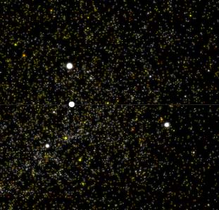
To make this, I downloaded public data from Hipparcos, a satellite launched by the European Space Agency in 1989 that accurately measured over a hundred thousand stars. The data I downloaded contains position, parallax, magnitude, and color information, among other things.

I used this information to plot the brightest stars, and cause them to revolve about Polaris (the North Star) very slowly, as the stars appear to do. Like the night sky, this is a sidereal time clock — it takes nearly 24 hours for the stars to fully rotate. You’ll notice some familiar constellations, such as the Big Dipper in there. As the stars cross zero and 180 degrees, indicated by the center line, the clock plays an individual note, or chime for each star. The pitch of the chime is based on the star’s BV measurement (which roughly corresponds to color or temperature). The volume is based on the star’s magnitude, or apparent brightness, and the stereo panning is based on the position on the screen (use headphones to hear it better).

Other projects that Bumgardner has developed include a music box that generates sound using trigonometry and harmonics and a camera that renders everything in ASCII code (yes, of course you can make yourself look like you’re in The Matrix). He also designed Coverpop, a program to which a user can give criteria that it uses to collects images and make a mosaic. All of these programs are more easily viewed and listened to than described, and are available on the Wheel of Stars site.

I interviewed Bumgardner about The Wheel of Stars via email. Here is what he had to say about the making of what he calls a “software toy”.

UT: What gave you the idea to make the Wheel of Stars?

JB: I’ve been interested in methods of producing automatic music since I studied music composition at CalArts. Among my interests are self-playing instruments like wind chimes, aeolian harps, player pianos and music boxes. A previous project which led directly to this one was my Whitney Music Box, based on the visual motion graphics of John Whitney.

So, already having the basic idea of using mathematical and random sources to trigger notes, in the style of a disc music box, it occurred to me that the stars themselves might make an interesting generator, and such a music box would make a very literal kind of “music of the spheres.”

UT: After looking at some of your other projects, I’m hard pressed as to exactly what to call the “Wheel of Stars.” It’s a toy, but more. It’s not really “just a software program,” or music visualizer, either. So, what do you call it?

JB: It’s a lot of things: It’s an aleatoric music composition which uses astronomical data for the “chance” element. It’s a software toy. It’s a work of art. It’s a musical clock. I think “software toy” is probably the best description from the above — a description I’ve applied to a lot of my projects. We hesitate to use the word “toy”, because we fear it belittles the project, but I think it imparts a healthy amount of playfulness in the description, and ultimately, these are works of play for me. I wrote a blog post which addresses this issue to some extent.

UT: I have to admit thinking, “This sounds what I have always imagined the “Music of the Spheres” to sound like.” You mention this in your description of the Wheel. This is probably a question you’ve had before, but I have to ask: was there any sort of influence from that age-old concept of the “Music of the Spheres” for the Wheel of Stars?

JB: Absolutely. My “Whitney Music Box” is another kind of music of the spheres, based as it is on basic trigonometry and harmonics. A lot of my work is concerned with circles, and I imagine I could go on making other kinds of “Music of the Spheres” for a long time to come.

I should also mention that the ethereal quality of the music is very much affected by my choice of audio sample. If I had used a Banjo sound, the effect would be quite different. I chose that particular sound because of my own preconceived notions of what a star should sound like. Probably a similar mental process to what Alexander Courage went through when he chose the opening notes for Star Trek.

UT: What would you like viewers/listeners to take away from the program/toy/visualizer?

JB: A little wonderment. A little more interest in the stars. Maybe do some research on Wikipedia, or pick up a good starter book like H.A. Rey’s “The Stars”. A very few listeners might be tempted to teach themselves how to program computers and make their own software toys. The “Processing” language is good place to start (processing.org).

UT: Have you had many planetariums or schools contact you to get it incorporated into their shows or curriculum?

JB: A couple nibbles, but nothing serious yet. I’d love to set up a large scale version of this piece — I think it would have a significant impact on the viewer.

UT: Did you design it with schools/planetariums in mind, or was it more for the pleasure of doing so?

JB: I made the piece because I was curious what it would sound like. Would it be totally random? Would there be hidden melodies or a secret message hidden in the stellar arrangement? Ultimately, I think I found a little bit of both. It’s quite different in character from what I would have gotten if the points where laid out with a number generator (and of course my choice of parameter mapping has a big effect on the outcome), but it’s not exactly morse code.

I also wanted to share it with people. The first version I made, in Processing, wasn’t easily sharable, so I ported it to Flash, so I could put it on the website.

UT: Any screen saver software planned for the future?

JB: I’ve prepared a stand-alone version which I email to folks upon request. It can be converted to a screen-saver with the right software. In my opinion, screensavers aren’t ideal for this kindof piece, because you don’t want your computer emitting sounds when you walk away (and can’t turn it off). But I think a stand-alone program that doesn’t require internet access, and which has higher quality sounds would be great.

UT: Do you plan to make any other astronomy-related programs like the Wheel of Stars?

JB: Yes. It occurs to me that a series of (8 or 9) short pieces based on astronomical data about the planets (their motions, and composition) might be interesting. However, at the moment, I’m pretty busy with other things.

UT: What other projects are you working on, astronomy-related or otherwise? I’ll cover the ASCII cam, Whitney Music Box and Coverpop and others in the article.

JB: I’m working on facilitating a showing of James Whitney’s extraordinary films “Lapis” and “Yantra” in Los Angeles next month (February 10th at the Silent Music Theater in Hollywood). We wlll be showing new digital transfers of these films, with live musical accompaniment. I also host and play piano at an Open Mic at Jones Coffee in Pasadena every month.

A couple of computer-related projects of interest: my recent music piece “Kasparov vs. Deep Blue” in which I programmed a chess computer to produce musical feedback showing what it is “thinking”, [See the video here] and my work simulating the automatic music algorithms of Athanasius Kircher. [a link to the paper can be found here].

Source: email interview with Jim Bumgardner. Cycling helmet nod to The Bad Astronomer

Stunning New Look at the Cat’s Paw Nebula

Cat's Paw Nebula. Credit: ESO

[/caption]

This striking new image shows the vast cloud of gas and dust known as the Cat’s Paw Nebula or NGC 6334. This glowing nebula resembles a gigantic pawprint of a celestial cat out on an errand across the Universe. This complex region of gas and dust, where numerous massive stars are born, lies near the heart of the Milky Way galaxy, about 5500 light-years away. It covers an area on the sky slightly larger than the full Moon. The whole gas cloud is about 50 light-years across.

This new portrait of the Cat’s Paw was created from images taken with the Wide Field Imager instrument at the 2.2-metre MPG/ESO telescope at the La Silla Observatory in Chile, combining images taken through blue, green and red filters, as well as a special filter designed to let through the light of glowing hydrogen.

The nebula appears red because its blue and green light are scattered and absorbed more efficiently by material between the nebula and Earth. The red light comes predominantly from hydrogen gas glowing under the intense glare of hot young stars.

Particularly striking is the red, intricate bubble in the lower right part of the image. This is most likely either a star expelling large amount of matter at high speed as it nears the end of its life or the remnant of a star that already has exploded.

NGC 6334 is one of the most active nurseries of massive stars in our galaxy and has been extensively studied by astronomers. The nebula conceals freshly minted brilliant blue stars — each nearly ten times the mass of our Sun and born in the last few million years. The region is also home to many baby stars that are buried deep in the dust, making them difficult to study. In total, the Cat’s Paw Nebula could contain several tens of thousands of stars.

Click here to see videos that pan and zoom into this stunning new image.