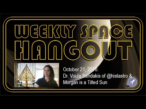
A razor thin Moon from October 22nd, 2014. Image credit and copyright: David Blanchflower.
This Halloween weekend’s top astronomical event features something that you won’t see in the sky.
By now, you’ve probably seen the stories circulating ’round ye ole web about how this month features a ‘Black Moon.’ The internet seems to love promulgating the passing of such curious calendrical oddities as Moons both Black, Blue and otherwise.
What’s all of the hoopla about? Well, simply put, the Moon reaches New phase this weekend on October 30th at 17:38 Universal Time (UT), marking the start of lunation 1161. This is the second New Moon for the month, as the first fell on October 1st, just 11 minutes into the month as reckoned in Universal Time.
Now, this isn’t at all rare or unusual; the synodic period of the Moon (that is, the time it takes to return to a similar phase, such as New back to New) is 29.5 days long, a period that shoehorns well in to a 31 day month like October, or occasionally, a 30 day month.
More Fun With Calendars
February is the only month that cannot contain a ‘repeat phase,’ leap year or no. Occasionally, a given phase such as New or Full can be absent from short February all together… sometimes, this oddity is also sometimes referred to as a ‘Black Moon.’ 2014 and 2033 are the nearest years to 2016 that are missing New Moons in February.
And then there’s the relict definition of a Blue Moon as the ‘3rd in an astronomical season with 4…‘ that can also be ascribed to a Black Moon as relates to New phase, as if we already lack enough multi-hued Moons in or lives.
Keep in mind, the moment of New is but an instant, a point a which the Moon’s longitude along the ecliptic plane equals the Sun’s. The Moon makes a miss of the Sun on most lunations, and only directly passes between the Sun and the Earth during an annular or solar eclipse. We’ve got one each coming up in 2017: an annular solar eclipse crossing the southern tip of South America on February 26th, and the historic return of totality to the United States on August 21st, 2017.
Said high profile solar eclipse next August also has a lesser role, as it fits that old-timey definition of the 3rd New Moon in an astronomical season with four. Of course, this is only the juxtaposition of the lunar cycle on our current Gregorian calendar, using time reckoned in UT/GMT.
Don’t fear the Black Moon. This year’s New Moon just misses Halloween. The next New Moon on Halloween (which, of course, is always a ‘Black Moon’) occurs in 2035.
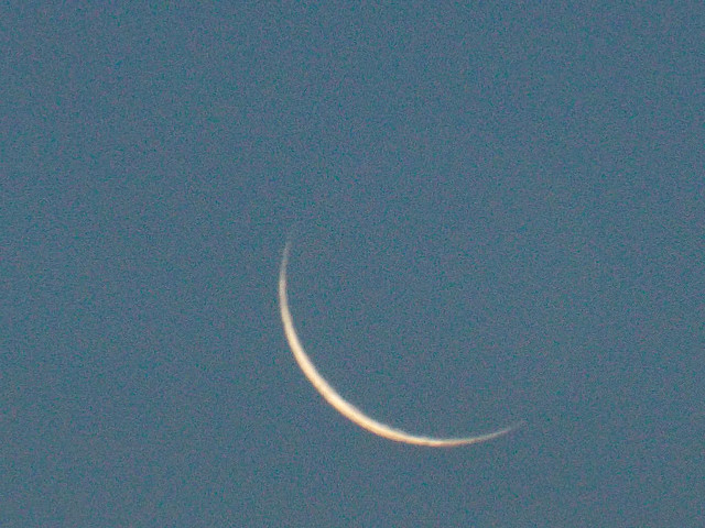
The view looking eastward on the morning of Friday, October 28th. Image credit: Stellarium
And we’ll let you in on a secret: astronomers don’t spend nights in mountaintop observatories discussing Black or Blue Moons… the term has more of an astrological tinge to it. Even in amateur astronomy circles, you sometimes hear the term ‘the dark of the Moon’ used to refer to the weeks surrounding New Moon, a prime time for deep sky astrophotography.
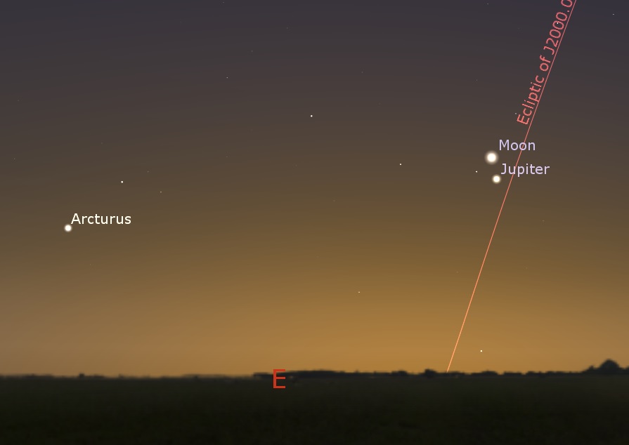
Looking for a New Moon-related observing challenge? Spotting the razor thin waxing or waning Moon is a fun feat of visual athletics. Look for a thin waning crescent Moon hanging near Jupiter on the morning of Friday, October 28th. This weekend, the first shot at catching the uber-thin Moon occurs for observers along a curve from southeastern Asia at dusk on October 31st westward at dusk. For Spain (and Astroguyz basecamp) the Moon will be 24 hours past New, and for the United States, the Moon will be 28 to 32 hours old at sunset for roaming Halloween ghouls and goblins, an easy catch.
First sighting opportunities for the waxing crescent Moon on Halloween evening. Graphic created by the author.
A time change is also afoot this weekend, as folks in Europe and the UK ‘fall back’ one hour to standard time. This setback falls nearly as late as it can in 2016, and we now enter that wacky oneeek period where the world slowly slips back to standard time. Blame ‘Big Sugar’ for the latency in most of North America, as prospective trick-or-treaters now make their rounds during daylight hours. In most of the US and Canada, the switch occurs on Sunday, November 6th.
And there’s one more astronomical tie-in for Halloween: the holiday traces its roots back as one of the four cross-quarter days of yore, including Lammas Day, Groundhog Day, and May Day. Of course, the fixing of Hallow’s Eve on October 31st makes the midway date only approximate: in 2016, the actual mid-point occurs on November 10th.
Out of this world stuff to consider, as you inventory the night’s sugary bounty and contemplate the night sky.
Artist's impression of The Milky Way Galaxy. Based on current estimates and exoplanet data, it is believed that there could be tens of billions of habitable planets out there. Credit: NASA
On a clear night, and when light pollution isn’t a serious factor, looking up at the sky is a breathtaking experience. On occasions like these, it is easy to be blown away by the sheer number of stars out there. But of course, what we can see on any given night is merely a fraction of the number of stars that actually exist within our Galaxy.
What is even more astounding is the notion that the majority of these stars have their own system of planets. For some time, astronomers have believed this to be the case, and ongoing research appears to confirm it. And this naturally raises the question, just how many planets are out there? In our galaxy alone, surely, there must be billions!
Number of Planets per Star:
To truly answer that question, we need to crunch some numbers and account for some assumptions. First, despite the discovery of thousands of extra-solar planets, the Solar System is still the only one that we have studied deeply. So it could be that ours possesses more star systems than others, or that our Sun has a fraction of the planets that other stars do.
So let’s assume that the eight planets that exist within our Solar System (not taking into account Dwarf Planets, Centaurs, KBOs and other larger bodies) represent an average. The next step will be to multiply that number by the amount of stars that exist within the Milky Way.
Number of Stars:
To be clear, the actual number of stars in the Milky Way is subject to some dispute. Essentially, astronomers are forced to make estimates due to the fact that we cannot view the Milky Way from the outside. And given that the Milky Way is in the shape of a barred, spiral disc, it is difficult for us to see from one side to the other – thanks to light interference from its many stars.
As a result, estimates of how many stars there are come down to calculations of our galaxy’s mass, and estimates of how much of that mass is made up of stars. Based on these calculations, scientists estimate that the Milky Way contains between 100 and 400 billion stars (though some think there could be as many as a trillion).
Doing the math, we can then say that the Milky Way galaxy has – on average – between 800 billion and 3.2 trillion planets, with some estimates placing that number as high a 8 trillion! However, in order to determine just how many of them are habitable, we need to consider the number of exoplanets discovered so far for the sake of a sample analysis.
Habitable Exoplanets:
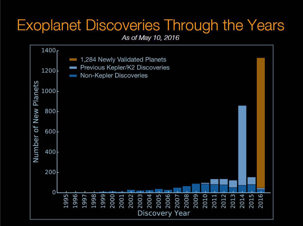
As of October 13th, 2016, astronomers have confirmed the presence of 3,397 exoplanets from a list of 4,696 potential candidates (which were discovered between 2009 and 2015). Some of these planets have been observed directly, in a process known as direct imaging. However, the vast majority have been detected indirectly using the radial velocity or transit method.
In the case of the former, the existence of planets is inferred based on the gravitational influence they have on their parent star. Essentially, astronomers measure how much the star moves back and forth to determine if it has a system of planets and how massive they are. In the case of the transit method, planets are detected when they pass directly in front of their star, causing it to dim. Here, size and mass are estimated based on the level of dimming.
In the course of its mission, the Kepler mission has observed about 150,000 stars, which during its initial four year mission consisted primarily of M-class stars. Also known as red dwarfs, these low-mass, lower-luminosity stars are harder to observe than our own Sun.
Histogram showing the number of exoplanets discovered by year. Credit: NASA Ames/W. Stenzel, Princeton/T. Morton
Since that time, Kepler has entered a new phase, also known as the K2 mission. During this phase, which began in November of 2013, Kepler has been shifting its focus to observe more in the way of K- and G-class stars – which are nearly as bright and hot as our Sun.
According to a recent study from NASA Ames Research Center, Kepler found that about 24% of M-class stars may harbor potentially habitable, Earth-size planets (i.e. those that are smaller than 1.6 times the radius of Earth’s). Based upon the number of M-class stars in the galaxy, that alone represents about 10 billion potentially habitable, Earth-like worlds.
Meanwhile, analyses of the K2 phase suggests that about one-quarter of the larger stars surveyed may also have Earth-size planet orbiting within their habitable zones. Taken together, the stars observed by Kepler make up about 70% of those found within the Milky Way. So one can estimate that there are literally tens of billions of potentially habitable planets in our galaxy alone.
In the coming years, new missions will be launching, like the James Webb Space Telescope (JWST) and the Transitting Exoplanet Survey Satellite (TESS). These missions will be able to detect smaller planets orbiting fainter stars, and maybe even determine if there’s life on any of them.
Once these new missions get going, we’ll have better estimates of the size and number of planets that orbit a typical star, and we’ll be able to come up with better estimates of just many planets there are in the galaxy. But until then, the numbers are still encouraging, as they indicate that the chances for extra-terrestrial intelligence are high!
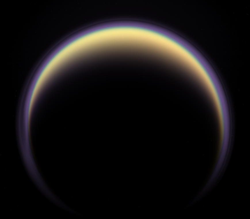
A halo of light surrounds Saturn's moon Titan in this backlit picture, showing its atmosphere. Credit: NASA/JPL/Space Science Institute
Ever since the Cassini probe arrived at Saturn in 2004, it has revealed some startling things about the planet’s system of moons. Titan, Saturn’s largest moon, has been a particular source of fascination. Between its methane lakes, hydrocarbon-rich atmosphere, and the presence of a “methane cycle” (similar to Earth’s “water cycle”), there is no shortage of fascinating things happening on this Cronian moon.
As if that wasn’t enough, Titan also experiences seasonal changes. At present, winter is beginning in the southern hemisphere, which is characterized by the presence of a strong vortex in the upper atmosphere above the south pole. This represents a reversal of what the Cassini probe witnessed when it first started observing the moon over a decade ago, when similar things were happening in the northern hemisphere.
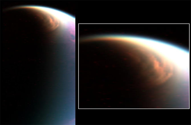
The large cloud in the stratosphere over Titan’s north pole (left) is similar to Earth’s polar stratospheric clouds (right). Credit: L. NASA/JPL/U. of Ariz./LPGNantes; R. NASA/GSFC/M. Schoeberl
During the course of the meeting, Dr. Athena Coustenis – the Director of Research (1st class) with the National Center for Scientific Research (CNRS) in France – shared the latest atmospheric data retrieved by Cassini. As she stated:
“Cassini’s long mission and frequent visits to Titan have allowed us to observe the pattern of seasonal changes on Titan, in exquisite detail, for the first time. We arrived at the northern mid-winter and have now had the opportunity to monitor Titan’s atmospheric response through two full seasons. Since the equinox, where both hemispheres received equal heating from the Sun, we have seen rapid changes.”
Scientists have been aware of seasonal change on Titan for some time. This is characterized by warm gases rising at the summer pole and cold gases settling down at the winter pole, with heat being circulated through the atmosphere from pole to pole. This cycle experiences periodic reversals as the seasons shift from one hemisphere to the other.
In 2009, Cassini observed a large scale reversal immediately after the equinox of that year. This led to a temperature drop of about 40 °C (104 °F) around the southern polar stratosphere, while the northern hemisphere experienced gradual warming. Within months of the equinox, a trace gas vortex appeared over the south pole that showed glowing patches, while a similar feature disappeared from the north pole.
High in the atmosphere of Titan, large patches of two trace gases glow near the north pole, on the dusk side of the moon, and near the south pole, on the dawn side. Credit: NRAO/AUI/NSF
A reversal like this is significant because it gives astronomers a chance to study Titan’s atmosphere in greater detail. Essentially, the southern polar vortex shows concentrations of trace gases – like complex hydrocarbons, methylacetylne and benzene – which accumulate in the absence of UV light. With winter now upon the southern hemisphere, these gases can be expected to accumulate in abundance.
As Coustenis explained, this is an opportunity for planetary scientists to test out their models for Titan’s atmosphere:
“We’ve had the chance to witness the onset of winter from the beginning and are approaching the peak time for these gas-production processes in the southern hemisphere. We are now looking for new molecules in the atmosphere above Titan’s south polar region that have been predicted by our computer models. Making these detections will help us understand the photochemistry going on.”
Previously, scientists had only been able to observe these gases at high northern latitudes, which persisted well into summer. They were expected to undergo slow photochemical destruction, where exposure to light would break them down depending on their chemical makeup. However, during the past few months, a zone of depleted molecular gas and aerosols has developed at an altitude of between 400 and 500 km across the entire northern hemisphere .
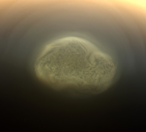
Titan’s south polar vortex. Credit: NASA/JPL-Caltech/Space Science Institute
This suggests that, at high altitudes, Titan’s atmosphere has some complex dynamics going on. What these could be is not yet clear, but those who have made the study of Titan’s atmosphere a priority are eager to find out. Between now and the end of Cassini mission (which is slated for Sept. 2017), it is expected that the probe will have provided a complete picture of how Titan’s middle and upper atmospheres behave.
By mission’s end, the Cassini space probe will have conducted more than 100 targeted flybys of Saturn. In so doing, it has effectively witnessed what a full year on Titan looks like, complete with seasonal variability. Not only will this information help us to understand the deeper mysteries of one of the Solar System’s most mysterious moons, it should also come in handy if and when we send astronauts (and maybe even settlers) there someday!
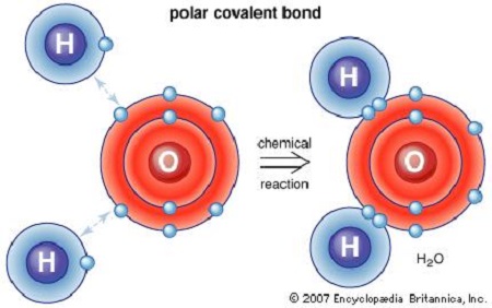
Water Molecules. Image Credit: National Science Foundation
For millennia, scientists have pondered the mystery of life – namely, what goes into making it? According to most ancient cultures, life and all existence was made up of the basic elements of nature – i.e. Earth, Air, Wind, Water, and Fire. However, in time, many philosophers began to put forth the notion that all things were composed of tiny, indivisible things that could neither be created nor destroyed (i.e. particles).
However, this was a largely philosophical notion, and it was not until the emergence of atomic theory and modern chemistry that scientists began to postulate that particles, when taken in combination, produced the basic building blocks of all things. Molecules, they called them, taken from the Latin “moles” (which means “mass” or “barrier”). But used in the context of modern particle theory, the term refers to small units of mass.
Definition:
By its classical definition, a molecule is the smallest particle of a substance that retains the chemical and physical properties of that substance. They are composed of two or more atoms, a group of like or different atoms held together by chemical forces.
Artist’s impression of simple and complex organic (carbon-containing) molecules that have been found in space. Credit: IAC/NASA/NOAO/ESA/Hubble Helix Nebula Team/M. Meixner/STScI/T.A. Rector/NRAO
It may consist of atoms of a single chemical element, as with oxygen (O2), or of different elements, as with water (H2O). As components of matter, molecules are common in organic substances (and therefore biochemistry) and are what allow for life-giving elements, like liquid water and breathable atmospheres.
Types of Bonds:
Molecules are held together by one of two types of bonds – covalent bonds or ionic bonds. A covalent bond is a chemical bond that involves the sharing of electron pairs between atoms. And the bond they form, which is the result of a stable balance of attractive and repulsive forces between atoms, is known as covalent bonding.
Ionic bonding, by contrast, is a type of chemical bond that involves the electrostatic attraction between oppositely charged ions. The ions involved in this kind of bond are atoms that have lost one or more electrons (called cations), and those that have gained one or more electrons (called anions). In contrast to covalence, this transfer is termed electrovalance.
In the simplest of forms, covelant bonds take place between a metal atom (as the cation) and a nonmetal atom (the anion), leading to compounds like Sodium Chloride (NaCl) or Iron Oxide (Fe²O³) – aka. salt and rust. However, more complex arrangements can be made too, such as ammonium (NH4+) or hydrocarbons like methane (CH4) and ethane (H³CCH³).
Diagram of a water molecule, which is made up of two hydrogen atoms and one oxygen atom. Credit: britannica.com
History of Study
Historically, molecular theory and atomic theory are intertwined. The first recorded mention of matter being made up of “discreet units” began in ancient India where practitioners of Jainism espoused the notion that all things were composed of small indivisible elements that combined to form more complex objects.
In ancient Greece, philosophers Leucippus and Democritus coined the term “atomos” when referring to the “smallest indivisible parts of matter”, from which we derive the modern term atom.
Then in 1661, naturalist Robert Boyle argued in a treatise on chemistry – titled “The Sceptical Chymist“- that matter was composed of various combinations of “corpuscules”, rather than earth, air, wind, water and fire. However. these observations were confined to the field of philosophy.
It was not until the late 18th and early 19th century when Antoine Lavoisier’s Law of Conservation of Mass and Dalton’s Law of Multiple Proportions brought atoms and molecules into the field of hard science. The former proposed that elements are basic substances that cannot be broken down further while the latter proposed that each element consists of a single, unique type, of atom and that these can join together to form chemical compounds.
Various atoms and molecules as depicted in John Dalton’s A New System of Chemical Philosophy (1808). Credit: Public Domain
A further boon came in 1865 when Johann Josef Loschmidt measured the size of the molecules that make up air, thus giving a sense of scale to molecules. The invention of the Scanning Tunneling Microscope (STM) in 1981 allowed for atoms and molecules to be observed directly for the first time as well.
Today, our concept of molecules is being refined further thanks to ongoing research in the fields of quantum physics, organic chemistry and biochemistry. And when it comes to the search for life on other worlds, an understanding of what organic molecules need in order to emerge from the combination of chemical building blocks, is essential.
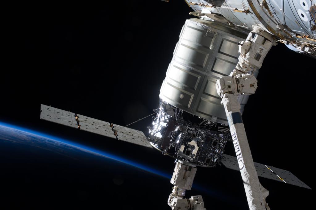
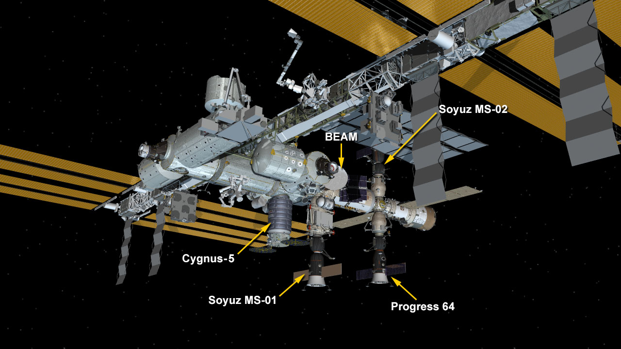
Installation complete! Orbital ATK's Cygnus cargo spacecraft was attached to the International Space_Station at 10:53 a.m. EDT on 23 Oct. 2016 after launching atop Antares rocket on 17 Oct. 2016 from NASA Wallops in Virginia. Credit: NASA
Installation complete! Orbital ATK’s Cygnus cargo spacecraft was attached to the International Space_Station at 10:53 a.m. EDT on 23 Oct. 2016 after launching atop Antares rocket on 17 Oct. 2016 from NASA Wallops in Virginia. Credit: NASA
After a two year gap, the first Cygnus cargo freight train from Virginia bound for the International Space Station (ISS) arrived earlier this morning – restoring this critical supply route to full operation today, Sunday, Oct. 23.
The Orbital ATK Cygnus cargo spacecraft packed with over 2.5 tons of supplies was berthed to an Earth-facing port on the Unity module of the ISS at 10:53 a.m. EDT.
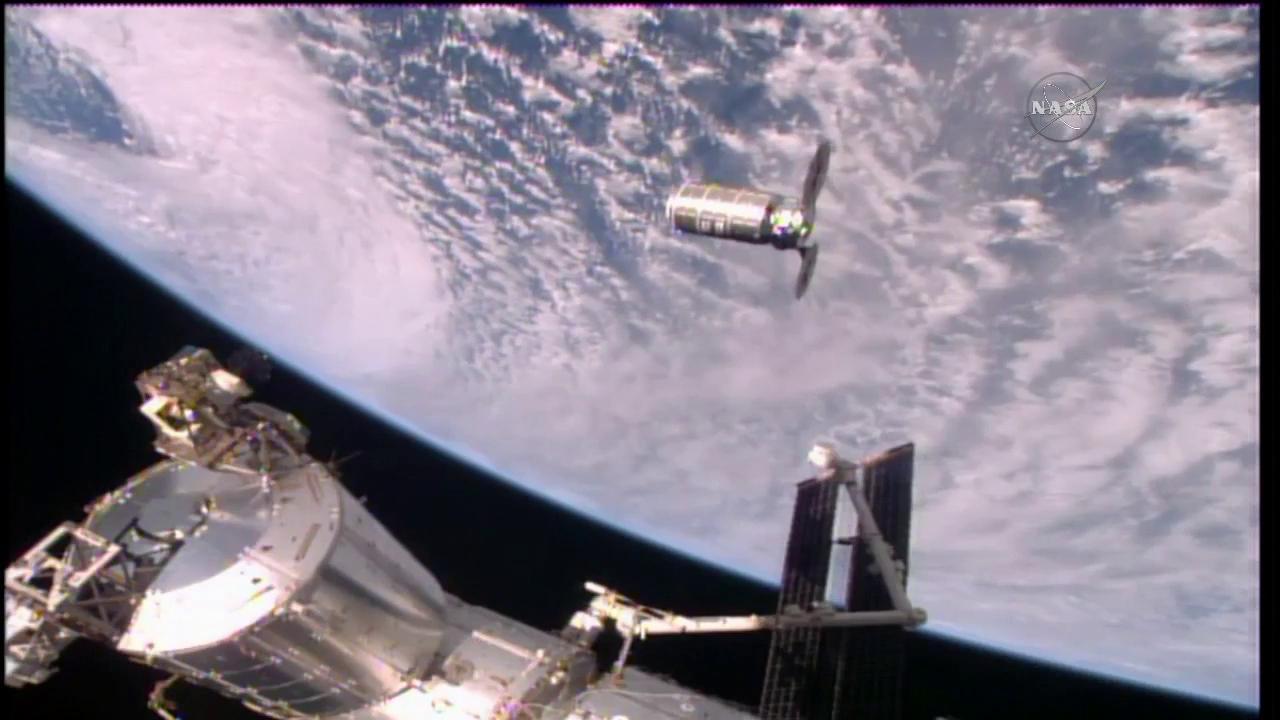
The Cygnus OA-5 resupply ship slowly approaches the space station before the Canadarm2 reaches out and grapples it on Oct. 23, 2016. Credit: NASA TV
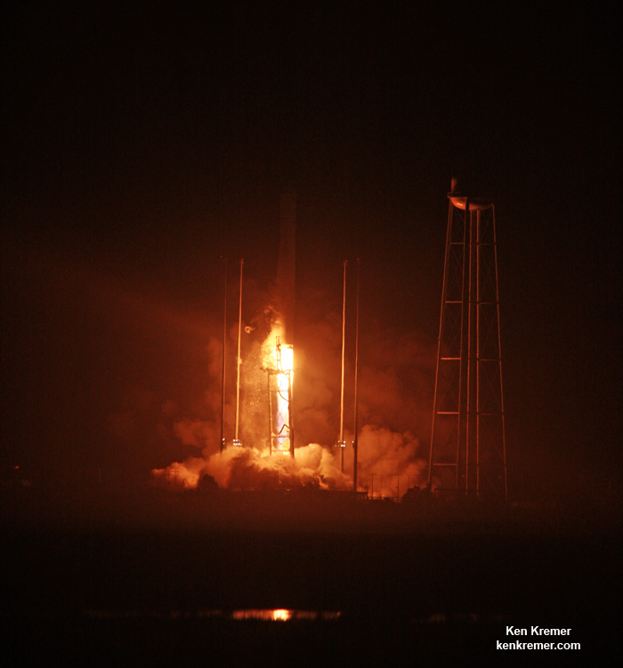
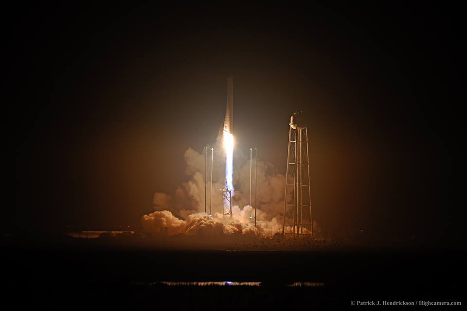
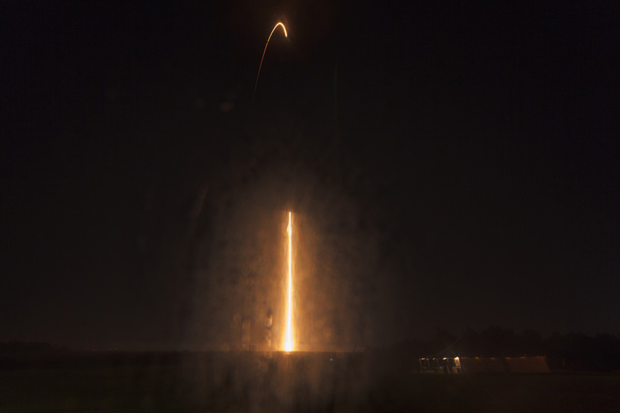
The Cygnus OA-5 mission took flight atop the first re-engined Orbital ATK Antares rocket during a spectacular Monday night liftoff on Oct. 17 at 7:40 p.m. EDT from the Mid-Atlantic Regional Spaceport pad 0A at NASA’s Wallops Flight Facility on Virginia’s picturesque Eastern shore.
Antares pair of RD-181 first stage engines were firing with some 1.2 million pounds of liftoff thrust and brilliantly lighting up the crystal clear evening skies in every direction to the delight of hordes of spectators gathered from near and far.
The Orbital ATK Antares rocket topped with the Cygnus cargo spacecraft launches from Pad-0A, Monday, Oct. 17, 2016 at NASA’s Wallops Flight Facility in Virginia. Orbital ATK’s sixth contracted cargo resupply mission with NASA to the International Space Station. Credit: Ken Kremer/kenkremer
Cygnus is loaded with over 5,100 pounds of science investigations, food, supplies and hardware for the space station and its six-person multinational crew.
This was the first Antares launch from Virginia in two years following the rockets catastrophic failure just moments after liftoff on Oct. 28, 2014, which doomed the Orb-3 resupply mission to the space station – as witnessed by this author.
Orbital ATK’s Antares commercial rocket had to be overhauled with the completely new RD-181 first stage engines- fueled by LOX/kerosene – following the destruction of the Antares rocket and Cygnus supply ship two years ago.
The 14 story tall commercial Antares rocket launched for the first time in the upgraded 230 configuration – powered by a pair of the new Russian-built RD-181 first stage engines.
The RD-181 replaces the previously used AJ26 engines which failed shortly after the last liftoff on Oct. 28, 2014 and destroyed the rocket and Cygnus cargo freighter.
The launch mishap was traced to a failure in the AJ26 first stage engine turbopump and forced Antares launches to immediately grind to a halt.
After a carefully choreographed five day orbital chase, Cygnus approached the million pound orbiting outpost this morning.
After it was within reach, Expedition 49 Flight Engineers Takuya Onishi of the Japan Aerospace Exploration Agency and Kate Rubins of NASA carefully maneuvered the station’s 57.7-foot (17.6-meter) Canadian-built robotic arm to reach out and capture the Cygnus OA-5 spacecraft at 7:28 a.m. EDT.
It was approximately 30 feet (10 meters) away from the station as Onishi and Rubins grappled the resupply ship with the robotic arms snares.
Today’s installation of the Orbital ATK Cygnus OA-5 resupply ship makes four spaceships attached to the International Space Station on 23 October 2016. Credit: NASA
After leak checks, the next step is for the crew to open the hatches between the pressurized Cygnus and Unity and begin unloading the stash aboard.
The 21-foot-long (6.4-meter) spacecraft is scheduled to spend about five weeks attached to the station. The crew will pack the ship with trash and no longer needed supplies and gear.
It will be undocked in November and then conduct several science experiments, including the Saffire fire experiment and deploy cubesats.
Thereafter it will be commanded to conduct the customary destructive re-entry in Earth’s atmosphere.
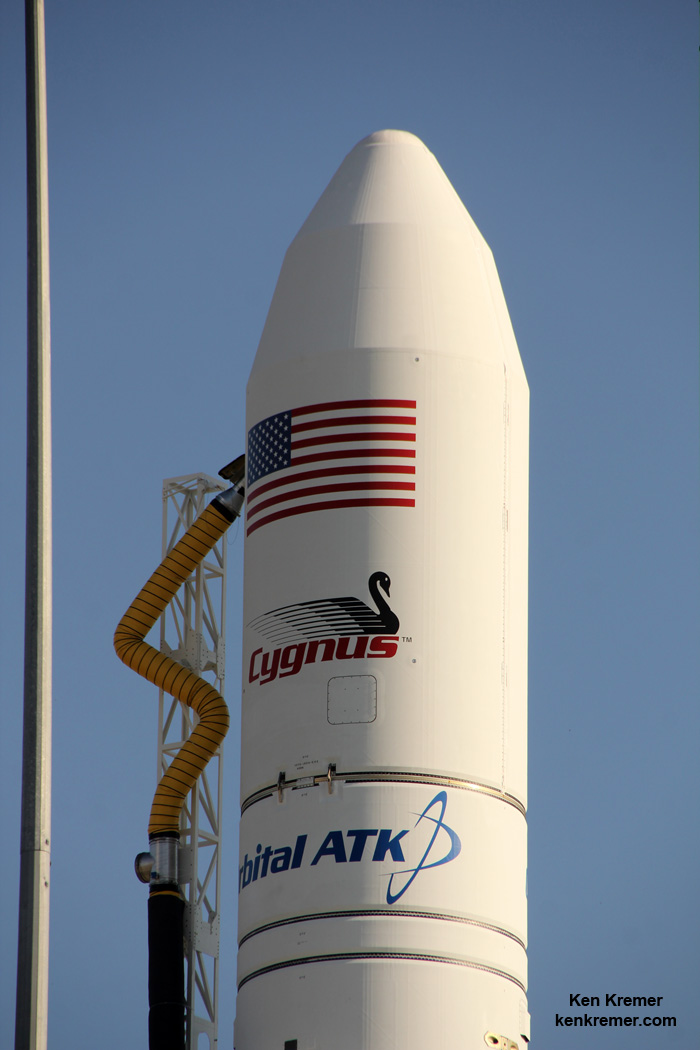
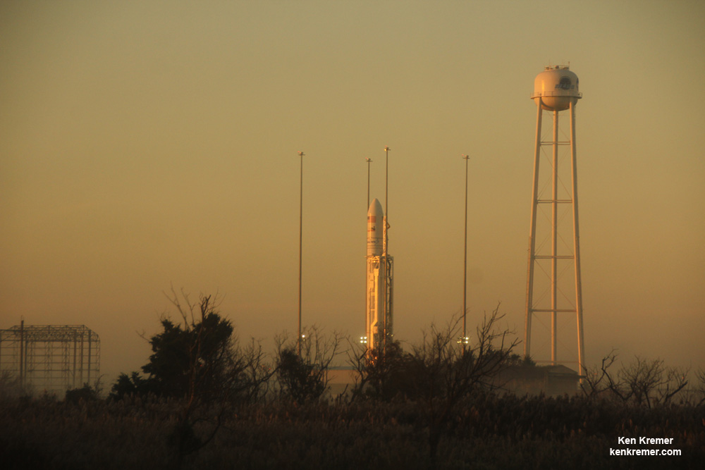
Cygnus cargo spacecraft atop Orbital ATK Antares rocket on Pad-0A prior to blastoff on Oct. 17, 2016 from NASA’s Wallops Flight Facility in Virginia on Orbital ATK’s sixth contracted cargo resupply mission with NASA to the International Space Station. Credit: Ken Kremer/kenkremer
The Cygnus spacecraft for the OA-5 mission is named the S.S. Alan G. Poindexter in honor of former astronaut and Naval Aviator Captain Alan Poindexter.
Under the Commercial Resupply Services (CRS) contract with NASA, Orbital ATK will deliver approximately 28,700 kilograms of cargo to the space station. OA-5 is the sixth of these missions.
Watch for Ken’s continuing Antares/Cygnus mission and launch reporting. He was reporting from on site at NASA’s Wallops Flight Facility, VA during the launch campaign.
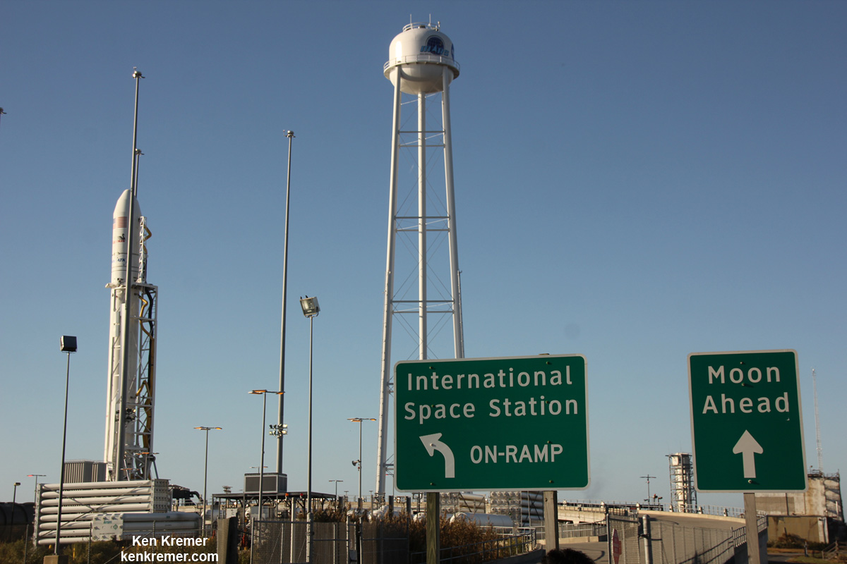
On-Ramp to the International Space Station (ISS) with Orbital ATL Antares rocket and Cygnus cargo freighter which launched on 17 Oct. 2016 and berthed at the Unity docking port on 23 Oct. 2016. Credit: Ken Kremer/kenkremer
Stay tuned here for Ken’s continuing Earth and Planetary science and human spaceflight news.
An Antares rocket sunrise prior to blastoff from NASA’s Wallops Flight Facility on 17 Oct. 2016 bound for the ISS. Credit: Ken Kremer/kenkremer Streak shot of Orbital ATK Antares rocket carrying Cygnus supply ship soars to orbit on Oct. 17, 2016 from Pad-0A at NASA’s Wallops Flight Facility in Virginia. Credit: Ken Kremer/kenkremer
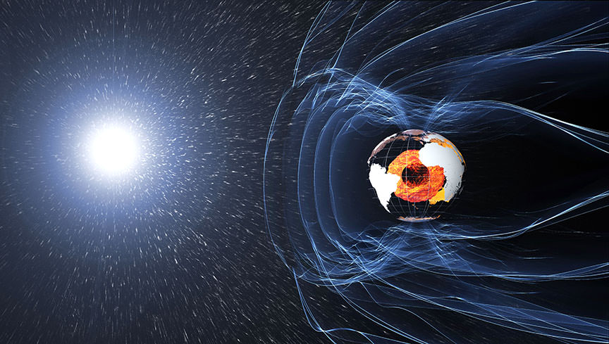
The magnetic field and electric currents in and around Earth generate complex forces that have immeasurable impact on every day life. Credit: ESA/ATG medialab
Everyone knows just how fun magnets can be. As a child, who among us didn’t love to see if we could make our silverware stick together? And how about those little magnetic rocks that we could arrange to form just about any shape because they stuck together? Well, magnetism is not just an endless source of fun or good for scientific experiments; it’s also one of basic physical laws upon which the universe is based.
The attraction known as magnetism occurs when a magnetic field is present, which is a field of force produced by a magnetic object or particle. It can also be produced by a changing electric field and is detected by the force it exerts on other magnetic materials. Hence why the area of study dealing with magnets is known as electromagnetism.
Definition:
Magnetic fields can be defined in a number of ways, depending on the context. However, in general terms, it is an invisible field that exerts magnetic force on substances which are sensitive to magnetism. Magnets also exert forces and torques on each other through the magnetic fields they create.
Visualization of the solar wind encountering Earth’s magnetosphere. Like a dipole magnet, it has field lines and a northern and southern pole. Credit: JPL
They can be generated within the vicinity of a magnet, by an electric current, or a changing electrical field. They are dipolar in nature, which means that they have both a north and south magnetic pole. The Standard International (SI) unit used to measure magnetic fields is the Tesla, while smaller magnetic fields are measured in terms of Gauss (1 Tesla = 10,000 Guass).
Mathematically, a magnetic field is defined in terms of the amount of force it exerted on a moving charge. The measurement of this force is consistent with the Lorentz Force Law, which can be expressed as F= qvB, where F is the magnetic force, q is the charge, v is the velocity, and the magnetic field is B. This relationship is a vector product, where F is perpendicular (->) to all other values.
Field Lines:
Magnetic fields may be represented by continuous lines of force (or magnetic flux) that emerge from north-seeking magnetic poles and enter south-seeking poles. The density of the lines indicate the magnitude of the field, being more concentrated at the poles (where the field is strong) and fanning out and weakening the farther they get from the poles.
A uniform magnetic field is represented by equally-spaced, parallel straight lines. These lines are continuous, forming closed loops that run from north to south, and looping around again. The direction of the magnetic field at any point is parallel to the direction of nearby field lines, and the local density of field lines can be made proportional to its strength.
Magnetic field lines resemble a fluid flow, in that they are streamlined and continuous, and more (or fewer lines) appear depending on how closely a field is observed. Field lines are useful as a representation of magnetic fields, allowing for many laws of magnetism (and electromagnetism) to be simplified and expressed in mathematical terms.
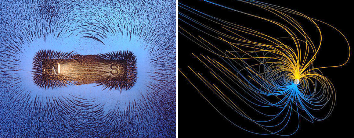
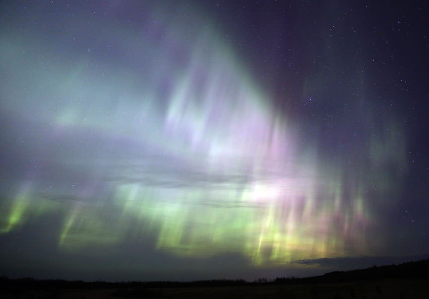
A simple way to observe a magnetic field is to place iron filings around an iron magnet. The arrangements of these filings will then correspond to the field lines, forming streaks that connect at the poles. They also appear during polar auroras, in which visible streaks of light line up with the local direction of the Earth’s magnetic field.
History of Study:
The study of magnetic fields began in 1269 when French scholar Petrus Peregrinus de Maricourt mapped out the magnetic field of a spherical magnet using iron needles. The places where these lines crossed he named “poles” (in reference to Earth’s poles), which he would go on to claim that all magnets possessed.
During the 16th century, English physicist and natural philosopher William Gilbert of Colchester replicated Peregrinus’ experiment. In 1600, he published his findings in a treaties (De Magnete) in which he stated that the Earth is a magnet. His work was intrinsic to establishing magnetism as a science.
View of the eastern sky during the peak of this morning’s aurora. Credit: Bob King
In 1750, English clergyman and philosopher John Michell stated that magnetic poles attract and repel each other. The force with which they do this, he observed, is inversely proportional to the square of the distance, otherwise known as the inverse square law.
In 1785, French physicist Charles-Augustin de Coulomb experimentally verified Earths’ magnetic field. This was followed by 19th century French mathematician and geometer Simeon Denis Poisson created the first model of the magnetic field, which he presented in 1824.
By the 19th century, further revelations refined and challenged previously-held notions. For example, in 1819, Danish physicist and chemist Hans Christian Orsted discovered that an electric current creates a magnetic field around it. In 1825, André-Marie Ampère proposed a model of magnetism where this force was due to perpetually flowing loops of current, instead of the dipoles of magnetic charge.
In 1831, English scientist Michael Faraday showed that a changing magnetic field generates an encircling electric field. In effect, he discovered electromagnetic induction, which was characterized by Faraday’s law of induction (aka. Faraday’s Law).
A Faraday cage in power plant in Heimbach, Germany. Credit: Wikipedia Commons/Frank Vincentz
Between 1861 and 1865, Scottish scientist James Clerk Maxwell published his theories on electricity and magnetism – known as the Maxwell’s Equations. These equations not only pointed to the interrelationship between electricity and magnetism, but showed how light itself is an electromagnetic wave.
The field of electrodynamics was extended further during the late 19th and 20th centuries. For instance, Albert Einstein (who proposed the Law of Special Relativity in 1905), showed that electric and magnetic fields are part of the same phenomena viewed from different reference frames. The emergence of quantum mechanics also led to the development of quantum electrodynamics (QED).
Examples:
A classic example of a magnetic field is the field created by an iron magnet. As previously mentioned, the magnetic field can be illustrated by surrounding it with iron filings, which will be attracted to its field lines and form in a looping formation around the poles.
Larger examples of magnetic fields include the Earth’s magnetic field, which resembles the field produced by a simple bar magnet. This field is believed to be the result of movement in the Earth’s core, which is divided between a solid inner core and molten outer core which rotates in the opposite direction of Earth. This creates a dynamo effect, which is believed to power Earth’s magnetic field (aka. magnetosphere).
Computer simulation of the Earth’s field in a period of normal polarity between reversals.[1] The lines represent magnetic field lines, blue when the field points towards the center and yellow when away. Credit: NASASuch a field is called a dipole field because it has two poles – north and south, located at either end of the magnet – where the strength of the field is at its maximum. At the midpoint between the poles the strength is half of its polar value, and extends tens of thousands of kilometers into space, forming the Earth’s magnetosphere.
Other celestial bodies have been shown to have magnetic fields of their own. This includes the gas and ice giants of the Solar System – Jupiter, Saturn, Uranus and Neptune. Jupiter’s magnetic field is 14 times as powerful as that of Earth, making it the strongest magnetic field of any planetary body. Jupiter’s moon Ganymede also has a magnetic field, and is the only moon in the Solar System known to have one.
Mars is believed to have once had a magnetic field similar to Earth’s, which was also the result of a dynamo effect in its interior. However, due to either a massive collision, or rapid cooling in its interior, Mars lost its magnetic field billions of years ago. It is because of this that Mars is believed to have lost most of its atmosphere, and the ability to maintain liquid water on its surface.
When it comes down to it, electromagnetism is a fundamental part of our Universe, right up there with nuclear forces and gravity. Understanding how it works, and where magnetic fields occur, is not only key to understanding how the Universe came to be, but may also help us to find life beyond Earth someday.
NASA's R5 "Valkyrie" robot may become a regular part of future crewed missions to Mars and beyond. Credit: NASA/B. Stafford/J. Blair/R. Geeseman
For over a decade, robots have been exploring Mars in advance of the crewed missions that are being planned for the coming decades. And when it comes time for astronauts to set foot on the Red Planet, they will be looking for robots to help them with some of the legwork. After all, exploring Mars is tough, laborious, and dangerous work, so some robotic assistance will probably be necessary.
For this reason, back in November of 2015, NASA gave the Massachusetts Institute of Technology one of their R5 “Valkyrie” humanoid robots. Since that time, MIT’s Computer Science and Artificial Intelligence Laboratory (CSAIL) has been developing special algorithms that will allow these robots to help out during future missions to Mars and beyond.
These efforts are being led Professor Russ Tedrake, an electrical engineer and computer programmer who helped program the Atlas robot to take part in the 2015 DARPA Robotics Challenge. Together with members of an advanced independent research group – known as the Super Undergraduate Research Opportunities Program (SuperUROP) – he is getting this R5 robot ready for NASA’s Space Robotics Challenge.
The DARPA Robotics Challenge (DRC) sought to inspire the creation of robots that could perform human tasks; in that case, for the sake of disaster relief. Credit: DARPA
As part of NASA’s Centennial Challenges Program, and with a prize purse of $1 million, this competition aims to push the boundaries of what robots are capable of in the realm of space exploration. In addition to MIT, Northeastern University and the University of Edinburgh have been tasked with programming an R5 to complete tasks normally handled by astronauts.
Ultimately, the robots will be tested in a simulated environment and judged based on their ability to complete three tasks. These include aligning a communications array, repairing a broken solar array, and identifying and repairing a habitat leak. There will also be a qualifying round where teams will be tasked with demonstrating autonomous tracking abilities (which will have to be completed in order to move towards the main round).
Naturally, this presents quite a few challenges. NASA designed the R5 robot to be capable of performing human tasks and move like a human being as much as possible, which necessitated a body with 28 torque-controlled joints. However, getting those joints to work together to perform mission-related work and operate independently is a bit of a challenge.
In short, the robot is not like other robotic missions – such as the Opportunity or Curiosity rovers. Instead of having a human being pushing levers to get them to move about and collect samples, the R5 will be tasked with things like opening airlock hatches, attaching and removing power cables, repairing equipment, and retrieving samples all on its own. And of course, if it takes a spill and falls down, it will have to be able to get up on its own.
NASA’s Space Robotics Challenge seeks to foster the development of robots that can help human astronauts during future missions, like to Mars. Credit: NASA/STMD
With the help of the special algorithms being generated by Tedrake and his colleagues – as well as other teams competing in this challenge – robots could play an important role in future missions. This could involve robots selecting landing sites for astronaut crews, setting up habitats in advance of crews arriving, and even conducting preliminary research on celestial bodies.
In addition, robots could take the place of crews on long-distance missions (such as Europa). Instead of sending a crew that would require months of food and supplies, a robot crew could be dispatched to the Jovian moon to collect ice samples, explore the surface, and interface with drones being sent to explore the interior ocean. And if the mission failed, there would be no grieving families (just grieving robotics teams).
And now to address the elephant in the room. The idea of sending robot explorers on space missions to help astronauts (or even replace them) is sure to make some people out there nervous. But for those who fear that this might bring one step closer to a robot revolution, rest assured that the machines are nowhere near where they’d need to be to go all “Judgement Day” on us just yet.
Long before they can launch nuclear weapons, pick up laser guns and stalk us through a post-apocalyptic landscape, or start upgrading themselves to look (and feel) human, robots will first need to master the simple tasks of walking upright and holding a screwdriver.
Still, if any of the robots end up having creepy red visor eyes (or saying things like “by your command”), we might want to consider including the Three Laws of Robotics in their programming. It’s never too soon to make sure they can’t turn on humanity!
Registration for the Space Robotics Challenge opened in August, 2016. The qualifying round, which began in mid-October, will run until mid-December. Finalists of that round will be announced in January, with the final virtual competition taking place in June 2017. The winning team will be awarded $500,000 over a two year period from NASA’s Space Technology Mission Directive.
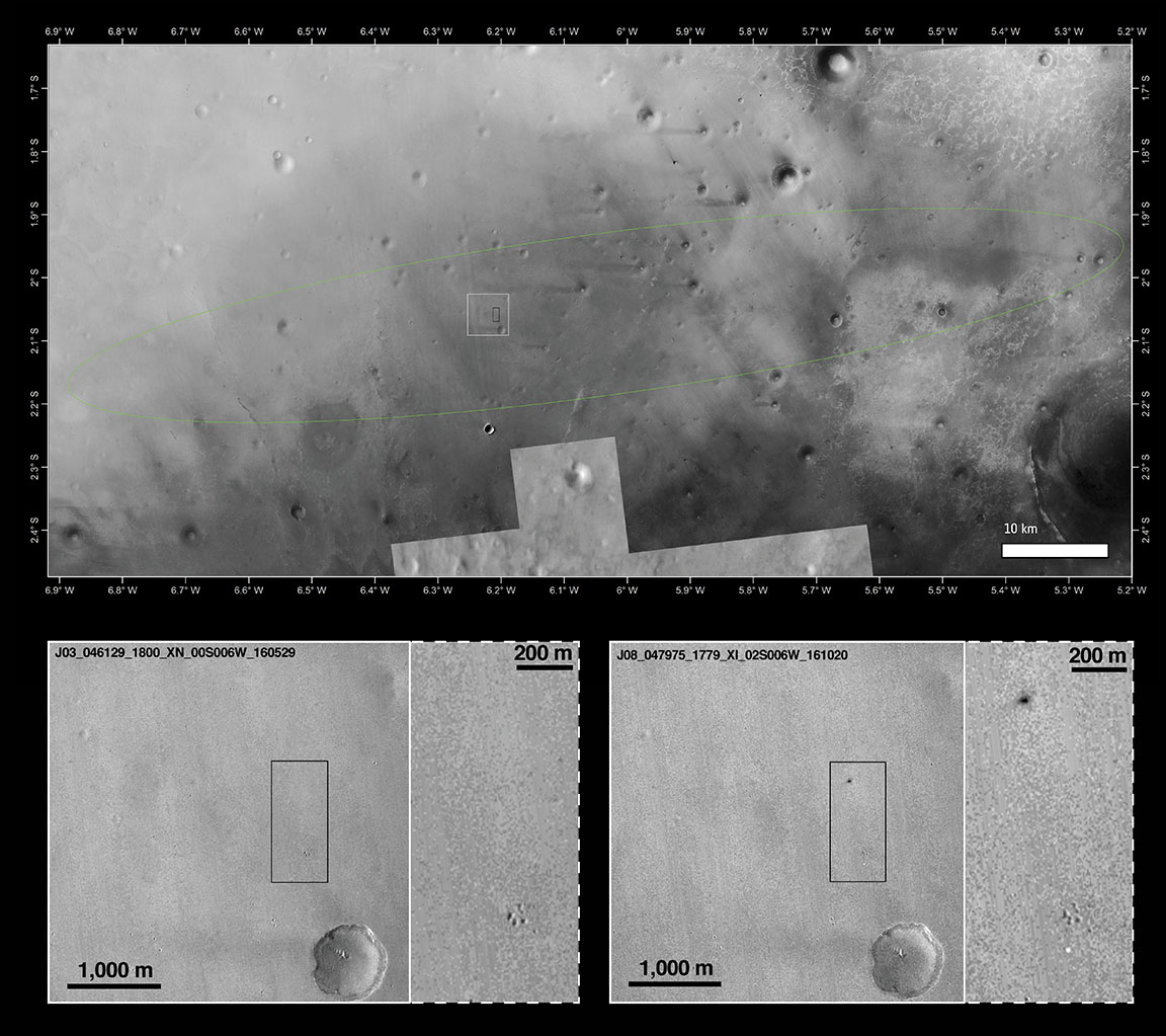
Mars Reconnaissance Orbiter view of Schiaparelli landing site before and after the lander arrived. The images have a resolution of 6 meters per pixel and shows two new features on the surface when compared to an image from the same camera taken in May this year. The black dot appears to be the lander impact site and the smaller white dot below the paw-shaped cluster of craters, the parachute. Credit: NASA
Mars Reconnaissance Orbiter view of Schiaparelli landing site before and after the lander arrived. The images have a resolution of 6 meters per pixel and shows two new features on the surface when compared to an image from the same camera taken in May this year. The black dot appears to be the lander impact site and the smaller white dot below the paw-shaped cluster of craters, the parachute. Credit: NASA
Instead of a controlled descent to the surface using its thrusters, ESA’s Schiaparelli lander hit the ground hard and may very well have exploded on impact. NASA’s Mars Reconnaissance Orbiter then-and-now photos of the landing site have identified new markings on the surface of the Red Planet that are believed connected to the ill-fated lander.
Schiaparelli entered the martian atmosphere at 10:42 a.m. EDT (14:42 GMT) on October 19 and began a 6-minute descent to the surface, but contact was lost shortly before expected touchdown seconds after the parachute and back cover were discarded. One day later, the Mars Reconnaissance Orbiter took photos of the expected touchdown site as part of a planned imaging run.
The landing site is shown within the Schiaparelli landing ellipse (top) along with before and after images below. Copyright Main image: NASA/JPL-Caltech/MSSS, Arizona State University; inserts: NASA/JPL-Caltech/MSSS
One of the features is bright and can be associated with the 39-foot-wide (12-meter) diameter parachute used in the second stage of Schiaparelli’s descent. The parachute and the associated back shield were released from Schiaparelli prior to the final phase, during which its nine thrusters should have slowed it to a standstill just above the surface.
The other new feature is a fuzzy dark patch or crater roughly 50 x 130 feet (15 x 40 meters) across and about 0.6 miles (1 km) north of the parachute. It’s believed to be the impact crater created by the Schiaparelli module following a much longer free fall than planned after the thrusters were switched off prematurely.
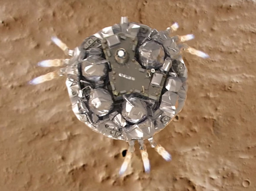
Artist’s concept of Schiaparelli deploying its parachute. The parachute may also have played a role in the crash. It may have deployed too soon, causing the thrusters to fire too soon. The thrusters may also have simply cut out too soon after firing. Credit: ESA
Mission control estimates that Schiaparelli dropped from between 1.2 and 2.5 miles (2 and 4 km) altitude, striking the Martian surface at more than 186 miles an hour (300 km/h). The dark spot is either disturbed surface material or it could also be due to the lander exploding on impact, since its thruster propellant tanks were likely still full. ESA cautions that these findings are still preliminary.
Something went wrong with Schiaparelli’s one or more sets of thrusters during the descent, causing the lander to crash on the surface at high speed. Credit: ESA
Since the module’s descent trajectory was observed from three different locations, the teams are confident that they will be able to reconstruct the chain of events with great accuracy. Exactly what happened to cause the thrusters to shut down prematurely isn’t yet known.
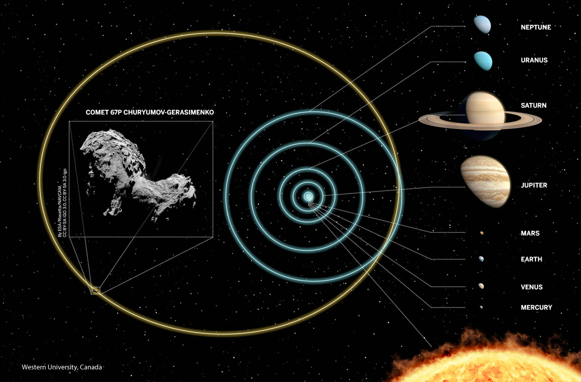
In the distant past, the orbit of 67P/Churyumov-Gerasimenko extended far beyond Neptune into the refrigerated Kuiper Belt. Interactions with the gravitational giant Jupiter altered the comet's orbit over time, dragging it into the inner Solar System. Credit: Western University, Canada
In the distant past, the orbit of 67P/Churyumov-Gerasimenko extended far beyond Neptune into the refrigerated Kuiper Belt. Interactions with the gravitational giant Jupiter altered the comet’s orbit over time, dragging it into the inner Solar System. Credit: Western University, Canada
Rosetta’s Comet hails from a cold, dark place. Using statistical analysis and scientific computing, astronomers at Western University in Canada have charted a path that most likely pinpoints comet 67P/Churyumov-Gerasimenko’s long-ago home in the far reaches of the Kuiper Belt, a vast region beyond Neptune home to icy asteroids and comets.
According to the new research, Rosetta’s Comet is relative newcomer to the inner parts of our Solar System, having only arrived about 10,000 years ago. Prior to that, it spent the last 4.5 billion years in cold storage in a rough-and-tumble region of the Kuiper Belt called the scattered disk.
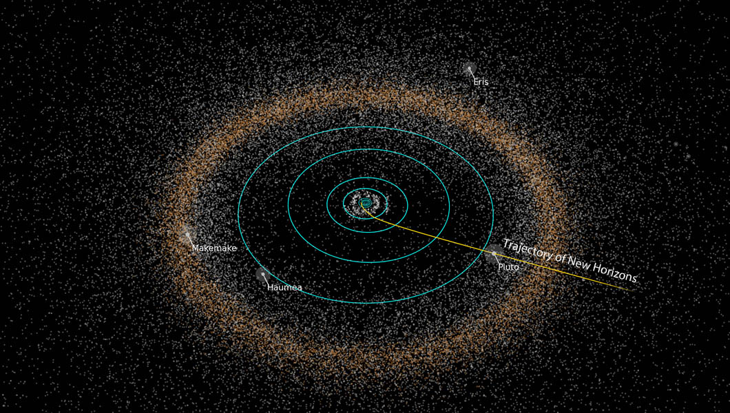
The Kuiper Belt was named in honor of Dutch-American astronomer Gerard Kuiper, who postulated a reservoir of icy bodies beyond Neptune. The first Kuiper Belt object was discovered in 1992. We now know of more than a thousand objects there, and it’s estimated it’s home to more than 100,000 asteroids and comets there over 62 miles (100 km) across. Credit: JHUAPL
In the Solar System’s youth, asteroids that strayed too close to Neptune were scattered by the encounter into the wild blue yonder of the disk. Their orbits still bear the scars of those long-ago encounters: they’re often highly-elongated (shaped like a cigar) and tilted willy-nilly from the ecliptic plane up to 40°. Because their orbits can take them hundreds of Earth-Sun distances into the deeps of space, scattered disk objects are among the coldest places in the Solar System with surface temperatures around 50° above absolute zero. Ices that glommed together to form 67P at its birth are little changed today. Primordial stuff.
Watch how Rosetta’s Comet’s orbit has evolved since the comet’s formation
There are two basic comet groups. Most comets reside in the cavernous Oort Cloud, a roughly spherical-shaped region of space between 10,000 and 100,000 AU (astronomical unit = one Earth-Sun distance) from the Sun. The other major group, the Jupiter-family comets, owes its allegiance to the powerful gravity of the giant planet Jupiter. These comets race around the Sun with periods of less than 20 years. It’s thought they originate from collisions betwixt rocky-icy asteroids in the Kuiper Belt.
Fragments flung from the collisions are perturbed by Neptune into long, cigar-shaped orbits that bring them near Jupiter, which ropes them like calves with its insatiable gravity and re-settles them into short-period orbits.
Comet 67P/Churyumov-Gerasimenko is a Jupiter-family comet. Its 6.5 year journey around the Sun takes it from just beyond the orbit of Jupiter at its most distant to between the orbits of Earth and Mars at its closest. Credit: ESA with labels by the author
Mattia Galiazzo and solar system expert Paul Wiegert, both at Western University, showed that in transit, Rosetta’s Comet likely spent millions of years in the scattered disk at about twice the distance of Neptune. The fact that it’s now a Jupiter family comet hints of a possible long-ago collision followed by gravitational interactions with Neptune and Jupiter before finally becoming an inner Solar System homebody going around the Sun every 6.45 years.
By such long paths do we arrive at our present circumstances.
Special Guest:
This week’s special guest is Dr. Voula Saridakis, a professor at Lake Forest College in Illinois specializing in the history of science and astronomy, who runsthe History of Astronomy on Twitter at @histastro
We use a tool called Trello to submit and vote on stories we would like to see covered each week, and then Fraser will be selecting the stories from there. Here is the link to the Trello WSH page (http://bit.ly/WSHVote), which you can see without logging in. If you’d like to vote, just create a login and help us decide what to cover!
If you would like to join the Weekly Space Hangout Crew, visit their site here and sign up. They’re a great team who can help you join our online discussions!
If you would like to sign up for the AstronomyCast Solar Eclipse Escape, where you can meet Fraser and Pamela, plus WSH Crew and other fans, visit our site linked above and sign up!
We record the Weekly Space Hangout every Friday at 12:00 pm Pacific / 3:00 pm Eastern. You can watch us live on Universe Today, or the Universe Today YouTube page.


![Computer simulation of the Earth's field in a period of normal polarity between reversals.[1] The lines represent magnetic field lines, blue when the field points towards the center and yellow when away. The rotation axis of the Earth is centered and vertical. The dense clusters of lines are within the Earth's core](https://www.universetoday.com/wp-content/uploads/2010/03/Geodynamo_Between_Reversals-e1449100829326.gif)