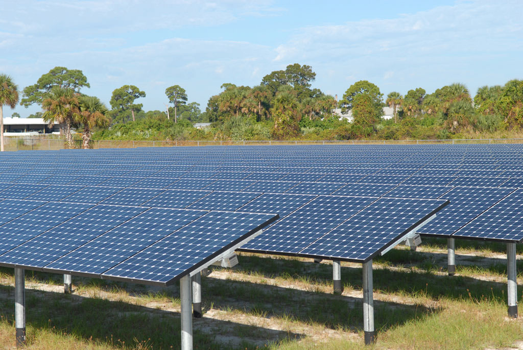
More than 3,300 solar panels have been erected on a vacant five acres at NASA's Kennedy Space Center. Credit: NASA/Jim Grossman
[/caption]
Today, the total oil and natural gas production provides about 60 percent of global energy consumption. This percentage is expected to peak about 10 to 30 years from now, and then be followed by a rapid decline, due to declining oil reserves and, hopefully, sources of renewable energy that technologies that will become more economically viable. But will there be the technology breakthroughs needed to make clean and exhaustible energy cost effective?
Nobel prize winner Walter Kohn, Ph.D., from the University of California Santa Barbara said that the continuous research and development of alternate energy could soon lead to a new era in human history in which two renewable sources — solar and wind — will become Earth’s dominant contributor of energy.
“These trends have created two unprecedented global challenges”, Kohn said, speaking at the American Chemical Society’s national meeting. “One is the threatened global shortage of acceptable energy. The other is the unacceptable, imminent danger of global warming and its consequences.”
The nations of the world need a concerted commitment to a changeover from the current era, dominated by oil plus natural gas, to a future era dominated by solar, wind, and alternative energy sources, Kohn said, and he sees that beginning to happen.
The global photovoltaic energy production increased by a factor of about 90 and wind energy by a factor of about 10 over the last decade. Kohn expects vigorous growth of these two energies to continue during the next decade and beyond, thereby leading to a new era, what he calls the SOL/WIND era, in human history, in which solar and wind energy have become the earth’s dominant alternative energies.
Kohn noted that this challenge require a variety of responses. “The most obvious is continuing scientific and technical progress providing abundant and affordable alternative energies, safe, clean and carbon-free,” he said.
One of the biggest challenges might be leveling off global population, as well as energy consumption levels.
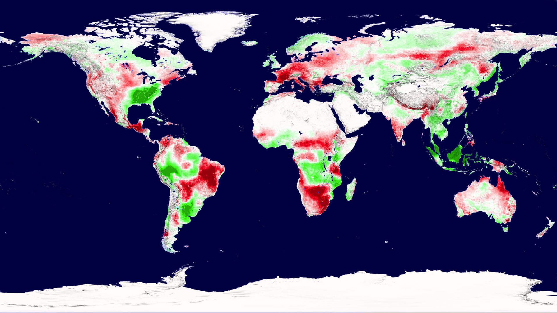
Caption: A snapshot of Earth's plant productivity in 2003 shows regions of increased productivity (green) and decreased productivity (red). Credit: NASA Goddard Space Flight Center Scientific Visualization Studio
[/caption]
One idea about climate change suggested that higher temperatures would boost plant growth and food production. That may have been a trend for awhile, where plant growth flourished with a longer growing season, but the latest analysis of satellite data shows that rising global temperatures has reached a tipping point where instead of being beneficial, higher temperatures are causing drought, which is now decreasing plant growth on a planetary scale. This could impact food security, biofuels, and the global carbon cycle. “This is a pretty serious warning that warmer temperatures are not going to endlessly improve plant growth,” said Steven Running from the University of Montana.
During the 1980s and 1990s global terrestrial plant productivity increased as much as six percent. Scientists say that happened because during that time, temperature, solar radiation and water availability — influenced by climate change — were favorable for growth.
During the past ten years, the decline in global plant growth is slight – just one percent. But it may signify a trend.
Interannual shifts in plant productivity (green line) fluctuated in step with shifts in atmospheric carbon dioxide (red line) between 2000 through 2009. Credit: Maosheng Zhao and Steven Running
“These results are extraordinarily significant because they show that the global net effect of climatic warming on the productivity of terrestrial vegetation need not be positive — as was documented for the 1980’s and 1990’s,” said Diane Wickland, of NASA Headquarters and manager of NASA’s Terrestrial Ecology research program.
A 2003 paper in Science led by then University of Montana scientist Ramakrishna Nemani (now at NASA Ames Research Center, Moffett Field, Calif.) showed that land plant productivity was on the rise.
Running and co-author Maosheng Zhao originally set out to update Nemani’s analysis, expecing to see similar results as global average temperatures have continued to climb. Instead, they found that the impact of regional drought overwhelmed the positive influence of a longer growing season, driving down global plant productivity between 2000 and 2009.
The discovery comes from an analysis of plant productivity data from the Moderate Resolution Imaging Spectroradiometer (MODIS) on NASA’s Terra satellite, combined with growing season climate variables including temperature, solar radiation and water. The plant and climate data are factored into an algorithm that describes constraints on plant growth at different geographical locations.
For example, growth is generally limited in high latitudes by temperature and in deserts by water. But regional limitations can vary in their degree of impact on growth throughout the growing season.
Zhao and Running’s analysis showed that since 2000, high-latitude northern hemisphere ecosystems have continued to benefit from warmer temperatures and a longer growing season. But that effect was offset by warming-associated drought that limited growth in the southern hemisphere, resulting in a net global loss of land productivity.
“This past decade’s net decline in terrestrial productivity illustrates that a complex interplay between temperature, rainfall, cloudiness, and carbon dioxide, probably in combination with other factors such as nutrients and land management, will determine future patterns and trends in productivity,” Wickland said.
The researchers plan on maintaining a record of the trends into the future. For one reason, plants act as a carbon dioxide “sink,” and shifting plant productivity is linked to shifting levels of the greenhouse gas in the atmosphere. Also, stresses on plant growth could challenge food production.
“The potential that future warming would cause additional declines does not bode well for the ability of the biosphere to support multiple societal demands for agricultural production, fiber needs, and increasingly, biofuel production,” Zhao said.
“Even if the declining trend of the past decade does not continue, managing forests and croplands for multiple benefits to include food production, biofuel harvest, and carbon storage may become exceedingly challenging in light of the possible impacts of such decadal-scale changes,” Wickland said.
The team published their findings Aug. 20 in Science.
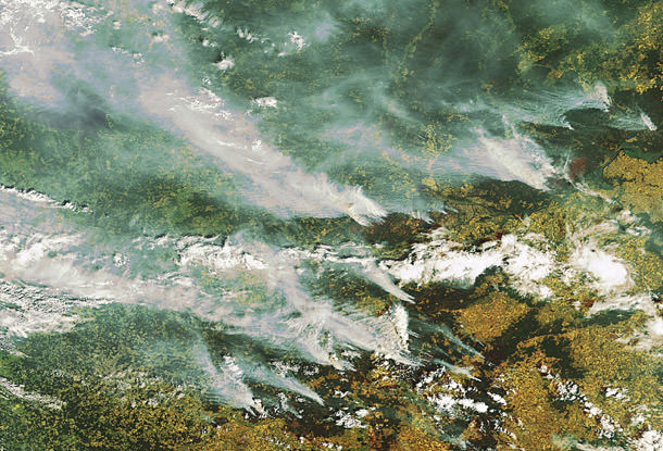
Wildfires in Russia as seen from space by ESA's Envisat satellite. Credit: ESA
[/caption]
Massive rains in Pakistan, China and Iowa in the US. Drought, heat and unprecedented fires in Russia and western Canada. 2010 is going down as the year of crazy, extreme weather. Is this just a wacky year or a trend of things to come? According to meteorologists, unusual holding patterns in the jet stream in the northern hemisphere are to blame for the extreme weather in Pakistan and Russia. But also, the World Meteorological Organization and other scientists say this type of weather fits patterns predicted by climate scientists, and could be the result of climate change.
“All these things are the kinds of things we would expect to happen as the planet warms up,” said Tom Wagner, a NASA scientist who studies the cryosphere, during an interview on CNN on August 11. “And we are seeing that the planet is warming about .35 degrees per decade. Places like Greenland are warming even faster, like 3.5 degrees per decade. And all these events from heat waves to stronger monsoons, to loss of ice are all consistent with that. Where it gets a little tricky is assigning any specific event to say, the cause of this event is definitely global warming, that is where we get to the edge of the research.”
“This weather is very unusual but there are always extremes every year,” said Andrew Watson from the University of East Anglia’s Environmental Studies. “We can never say that weather in a single year is unequivocal evidence of climate change, if you get many years of extreme weather then that can point to climate change.”
The Intergovernmental Panel on Climate Change (IPCC) has long predicted that rising global temperatures would produce more frequent and intense heat waves, and more severe rainfalls. In its 2007 report, the panel said these trends have already been observed, with an increase in heat waves since 1950, for example.
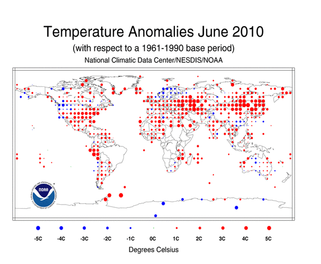
NOAA measurements show that the combined global surface temperatures for June 2010 are the warmest on record, and Wagner said there are larger conclusions to be drawn from the definite global warming trend. “We are seeing things that haven’t really happened before on the planet, like warming at this specific rate. We think it is very well tied to increasing carbon dioxide in the atmosphere since the late 1800’s caused by humans.”
This graph, based on the comparison of atmospheric samples contained in ice cores and more recent direct measurements, provides evidence that atmospheric CO2 has increased since the Industrial Revolution. (Source: NOAA)
“Not just over 10 years, but we have satellites images, weather station records and other good records going back to the late 1800’s that tells us all about how the planet is warming up,” Wagner said. “Not only that but we have evidence from geologic records, ice cores, and sediment cores from ocean cores. All of this feeds together to show us how the planet is changing.”
Asked if the cycle can be reversed, Wagner replied, “That is the million dollar question. One thing we have to think about is that the planet is changing and we have to deal with that. Ice around Antarctica and Greenland is melting. Sea level is rising right now at 3 millimeters a year. If you just extrapolate that to 100 years, it will rise to at least a foot of sea level rise. But there is the possibility it could be more than that. These are the types of things we need to think about and come up with mitigation strategies to deal with them. We’re doing the research to try and nail down these questions a little more tightly to see how much sea level is going to rise, how much temperatures are going to rise and how are weather patterns going to change.”
Reducing emissions is one thing that everyone can do to help protect the planet and the climate, and climate experts have been saying for years that there needs to be sharp cutbacks in emissions of carbon dioxide and other heat-trapping gases that go into the atmosphere from automobiles, power plants, and other fossil fuel-burning industrial and residential sources.
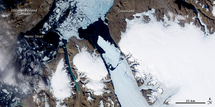
In the news this week was the huge ice chunk coming loose from a Greenland glacier. Not only is this an indication of warming water, but other problems could develop, such as the large ice chunks getting in the way of shipping lanes or heading towards oil rigs. The high temperatures and fires in Russia are affecting big percentage of the world’s wheat production, and could have an effect on our food supply this coming year.
Not only that, but the wildfires have created a noxious soup of air pollution that is affecting life far beyond just the local regions, JPL reports. Among the pollutants created by wildfires is carbon monoxide, a gas that can pose a variety of health risks at ground level. Carbon monoxide is also an ingredient in the production of ground-level ozone, which causes numerous respiratory problems. As the carbon monoxide from these wildfires is lofted into the atmosphere, it becomes caught in the lower bounds of the mid-latitude jet stream, which swiftly transports it around the globe.
Two movies were created using continuously updated data from the “Eyes on the Earth 3-D” feature, also on NASA’s global climate change website. They show three-day running averages of daily measurements of carbon monoxide present at an altitude of 5.5 kilometers (18,000) feet, along with its global transport.
And in case you are wondering, the recent solar flares have nothing to do with the wildfires — as Ian O’Neill from Discovery space deftly points out.
Enormous chuck of ice breaks off the Petermann Glacier in Greenland. Credit: NASA.
[/caption]
A huge ice island four times the size of Manhattan– and half as thick as the Empire State Building is tall– has broken off from one of Greenland’s two main glaciers. On August 5, 2010, an enormous chunk of ice, roughly 97 square miles (251 square kilometers) in size, broke off the Petermann Glacier, along the northwestern coast of Greenland. Satellite images, like this one from NASA’s Aqua satellite show the glacier lost about one-quarter of its 70-kilometer (40-mile) long floating ice shelf. Located a thousand kilometers south of the North Pole, the now-separate ice island contains enough fresh water to keep public tap water in the United States flowing for 120 days, said scientists from the University of Delaware who have been monitoring the break.
While thousands of icebergs detach from Greenland’s glaciers every year, the last time one this large formed was in 1962. The flow of sea water beneath Greenland’s glaciers is a main cause of ice detaching from them.
This movie made from another satellite — Envisat from the European Space Agency – shows the giant iceberg breaking off.
Time-series animation based on Envisat Advanced Synthetic Aperture Radar (ASAR) data from 31 July, 4 August, and 7 August 2010 showing the breaking of the Petermann glacier and the movement of the new iceberg towards Nares Strait. Credits: ESA
The animation above was created by combining three Advanced Synthetic Aperture Radar (ASAR) acquisitions (31 July, 4 August and 7 August 2010) taken over the same area. The breaking of the glacier tongue and the movement of the iceberg can be clearly seen in this sequence.
The Petermann glacier is one of the largest glaciers connecting the Greenland inland ice sheet with the Arctic Ocean. Upon reaching the sea, a number of these large outlet glaciers extend into the water with a floating ‘ice tongue’.
The ice tongue of the Petermann glacier was the largest in Greenland. This tide-water glacier regularly advances towards the ocean at about 1 km per year. During the previous months, satellite images revealed that several cracks had appeared on the glacier surface, suggesting to scientists that a break-up event was imminent.
Scientists say it’s hard to tell if global warming caused the event. Records on the glacier and sea water below have only been kept since 2003. The first six months of 2010 have been the hottest globally on record.
June Land Surface Temperature Anomalies in degrees Celsius. Credit: NOAA
[/caption]
Was last month warm where you live? If so, you weren’t alone. According measurements taken by the National Oceanic and Atmospheric Administration (NOAA) June 2010 was the hottest June on record worldwide. But this is not a new trend, at least for this year. March, April, and May 2010 were also the warmest on record. This was also the 304th consecutive month with a global temperature above the 20th century average. The last month with below-average temperature was February 1985.
Here are some of the numbers:
* The combined global land and ocean average surface temperature for June 2010 was the warmest on record at 16.2°C (61.1°F), which is 0.68°C (1.22°F) above the 20th century average of 15.5°C (59.9°F). The previous record for June was set in 2005.
* The June worldwide averaged land surface temperature was 1.07°C (1.93°F) above the 20th century average of 13.3°C (55.9°F)—the warmest on record.
* It was the warmest April–June (three-month period) on record for the global land and ocean temperature and the land-only temperature. The three-month period was the second warmest for the world’s oceans, behind 1998.
* It was the warmest June and April–June on record for the Northern Hemisphere as a whole and all land areas of the Northern Hemisphere.
* It was the warmest January–June on record for the global land and ocean temperature. The worldwide land on average had its second warmest January–June, behind 2007. The worldwide averaged ocean temperature was the second warmest January–June, behind 1998.
* Sea surface temperature (SST) anomalies in the central and eastern equatorial Pacific Ocean continued to decrease during June 2010. According to NOAA’s Climate Prediction Center, La Niña conditions are likely to develop during the Northern Hemisphere summer 2010.
Some regions on the planet, however, had cool temps for a northern hemisphere summer. Spain had its coolest June temperatures since 1997, and Guizhou in southern China had its coolest June since their records began in 1951.
Still, with those cool temperatures, the planet on the whole was warmer.
Arctic sea ice extent for June 2010 was 10.87 million square kilometers (4.20 million square miles). Credit: NSIDC
Other satellite data from the US National Snow and Ice Data Center in Colorado shows that the extent of sea ice in the Arctic was at its lowest for any June since satellite records started in 1979. The ice cover on Arctic Ocean grows each winter and shrinks in summer, reaching its annual low point in September. The monthly average for June 2010 was 10.87 km sq. The ice was declining an average of 88,000 sq km per day in June. This rate of decline is the fastest measured for June.
During June, ice extent was below average everywhere except in the East Greenland Sea, where it was near average.
We keep finding all these exoplanets. Our detection methods still only pick out the bigger ones, but we’re getting better at this all the time. One day in the not-too-distant future it is conceivable that we will find one with a surface gravity in the 1G range – orbiting its star in, what we anthropomorphically call, the Goldilocks zone where water can exist in liquid phase.
So let’s say we find such a planet and then direct all our SETI gear towards it. We start detecting faint morse-code like beeps – inscrutable, but clearly of artificial origin. Knowing us, we’ll send out a probe. Knowing us, there will be a letter campaign demanding that we adhere to the Prime Directive and consequently this deep space probe will include some newly developed cloaking technology, so that it will arrive at the Goldilocks planet invisible and undetectable.
The probe takes quite a while to get there and, in transit, receives indications that the alien civilization is steadily advancing its technology as black and white sitcoms start coming through – and as all that is relayed back to us we are able to begin translating their communications into a range of ‘dialects’.
By the time the probe has arrived and settles into an invisible orbit, it’s apparent a problem is emerging on the planet. Many of its inhabitants have begun expressing concern that their advancing technology is beginning to have planetary effects, with respect to land clearing and atmospheric carbon loading.
From our distant and detached viewpoint we are able to see that anyone on the planet who thinks they live in a stable and unchanging environment just isn’t paying attention. There was a volcano just the other week and their geologists keep finding ancient impact craters which have revised whole ecosystems in their planet’s past.
It becomes apparent that the planet’s inhabitants are too close the issues to be able to make a dispassionate assessment about what’s happening – or what to do about it. They are right that their technological advancement has bumped up the CO2 levels from 280ppm to over 380ppm within only 150 years – and to a level much higher than anything detectable in their ice core data, which goes back half a million years. But that’s about where the definitive data ends.
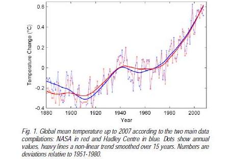
Credit: Rahstorf. NASA data is from the GISS Surface Temperature Analysis. Hadley Centre data is from the Met Office Hadley Centre, UK.
Advocates for change draw graphs showing temperatures are rising, while conservatives argue this is just cherry-picking data from narrow time periods. After all, a brief rise might be lost in the background noise of a longer monitoring period – and just how reliable is 150 year old data anyway? Other more pragmatic individuals point to the benefits gained from their advanced technology, noting that you have to break a few eggs to make an omelet (or at least the equivalent alien cuisine).
Back on Earth our future selves smile wryly, having seen it all before. As well as interstellar probes and cloaking devices, we have developed a reliable form of Asimovian psychohistory. With this, it’s easy enough to calculate that the statistical probability of a global population adopting a coordinated risk management strategy in the absence of definitive, face-slapping evidence of an approaching calamity is exactly (datum removed to prevent corrupting the timeline).
For Goldilocks, the porridge had to be not too hot, and not too cold … the right temperature was all she needed.
For an Earth-like planet to harbor life, or multicellular life, certainly temperature is important, but what else is important? And what makes the temperature of an exo-Earth “just right”?
Some recent studies have concluded that answering these questions can be surprisingly difficult, and that some of the answers are surprisingly curious.
Consider the tilt of an exo-Earth’s axis, its obliquity.
In the “Rare Earth” hypothesis, this is a Goldilocks criterion; unless the tilt is kept stable (by a moon like our Moon), and at a “just right” angle, the climates will swing too wildly for multicellular life to form: too many snowball Earths (the whole globe covered in snow and ice with an enhanced albedo effect), or too much risk of a runaway greenhouse.
“We find that planets with small ocean fractions or polar continents can experience very severe seasonal climatic variations,” Columbia University’s David Spiegel writes*, summing up the results of an extensive series of models investigating the effects of obliquity, land/ocean coverage, and rotation on Earth-like planets, “but that these planets also might maintain seasonally and regionally habitable conditions over a larger range of orbital radii than more Earth-like planets.” And the real surprise? “Our results provide indications that the modeled climates are somewhat less prone to dynamical snowball transitions at high obliquity.” In other words, an exo-Earth tilted nearly right over (much like Uranus) may be less likely to suffer snowball Earth events than our, Goldilocks, Earth! Ultraviolet view of the Sun. Image credit: SOHO
Consider ultra-violet radiation.
“Ultraviolet radiation is a double-edged sword to life. If it is too strong, the terrestrial biological systems will be damaged. And if it is too weak, the synthesis of many biochemical compounds cannot go along,” says Jianpo Guo of China’s Yunnan Observatory** “For the host stars with effective temperatures lower than 4,600 K, the ultraviolet habitable zones are closer than the habitable zones. For the host stars with effective temperatures higher than 7,137 K, the ultraviolet habitable zones are farther than the habitable zones.” This result doesn’t change what we already knew about habitability zones around main sequence stars, but it effectively rules out the possibility of life on planets around post-red giant stars (assuming any could survive their homesun going red giant!) (Credit: NASA)
Consider the effects of clouds.
Calculations of the habitability zones – the radii of the orbits of an exo-Earth, around its homesun – for main sequence stars usually assume an astronomers’ heaven – permanent clear skies (i.e. no clouds). But Earth has clouds, and clouds most definitely have an effect on average global temperatures! “The albedo effect is only weakly dependent on the incident stellar spectra because the optical properties (especially the scattering albedo) remain almost constant in the wavelength range of the maximum of the incident stellar radiation,” a German team’s recent study*** on the effects of clouds on habitability concludes (they looked at main sequence homesuns of spectral classes F, G, K, and M). This sounds like Gaia is Goldilocks’ friend; however, “The greenhouse effect of the high-level cloud on the other hand depends on the temperatures of the lower atmosphere, which in turn are an indirect consequence of the different types of central stars,” the team concludes (remember that an exo-Earth’s global temperature depends upon both the albedo and greenhouse effects). So, the take-home message? “Planets with Earth-like clouds in their atmospheres can be located closer to the central star or farther away compared to planets with clear sky atmospheres. The change in distance depends on the type of cloud. In general, low-level clouds result in a decrease of distance because of their albedo effect, while the high-level clouds lead to an increase in distance.”
“Just right” is tricky to pin down.
* lead author; Princeton University’s Kristen Manou and Colombia University’s Caleb Scharf are the co-authors (“Habitable Climates: The Influence of Obliquity”, The Astrophysical Journal, Volume 691, Issue 1, pp. 596-610 (2009); arXiv:0807.4180 is the preprint)
** lead author; Fenghui Zhang, Xianfei Zhang, and Zhanwen Han, all also at the Yunnan Observatory, are the co-authors (“Habitable zones and UV habitable zones around host stars”, Astrophysics and Space Science, Volume 325, Number 1, pp. 25-30 (2010))
*** “Clouds in the atmospheres of extrasolar planets. I. Climatic effects of multi-layered clouds for Earth-like planets and implications for habitable zones”, Kitzmann et al., accepted for publication in Astronomy & Astrophysics (2010); arXiv:1002.2927 is the preprint.
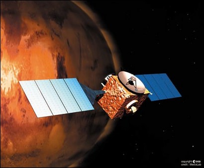
An illustration showing the ESA's Mars Express mission. Credit: ESA/Medialab)
Understanding the present-day Martian climate gives us insights into its past climate, which in turn provides a science-based context for answering questions about the possibility of life on ancient Mars.
Our understanding of Mars’ climate today is neatly packaged as climate models, which in turn provide powerful consistency checks – and sources of inspiration – for the climate models which describe anthropogenic global warming here on Earth.
But how can we work out what the climate on Mars is, today? A new, coordinated observation campaign to measure ozone in the Martian atmosphere gives us, the interested public, our own window into just how painstaking – yet exciting – the scientific grunt work can be.
[/caption]
The Martian atmosphere has played a key role in shaping the planet’s history and surface. Observations of the key atmospheric components are essential for the development of accurate models of the Martian climate. These in turn are needed to better understand if climate conditions in the past may have supported liquid water, and for optimizing the design of future surface-based assets at Mars.
Ozone is an important tracer of photochemical processes in the atmosphere of Mars. Its abundance, which can be derived from the molecule’s characteristic absorption spectroscopy features in spectra of the atmosphere, is intricately linked to that of other constituents and it is an important indicator of atmospheric chemistry. To test predictions by current models of photochemical processes and general atmospheric circulation patterns, observations of spatial and temporal ozone variations are required.
The Spectroscopy for Investigation of Characteristics of the Atmosphere of Mars (SPICAM) instrument on Mars Express has been measuring ozone abundances in the Martian atmosphere since 2003, gradually building up a global picture as the spacecraft orbits the planet.
These measurements can be complemented by ground-based observations taken at different times and probing different sites on Mars, thereby extending the spatial and temporal coverage of the SPICAM measurements. To quantitatively link the ground-based observations with those by Mars Express, coordinated campaigns are set up to obtain simultaneous measurements.
Infrared heterodyne spectroscopy, such as that provided by the Heterodyne Instrument for Planetary Wind and Composition (HIPWAC), provides the only direct access to ozone on Mars with ground-based telescopes; the very high spectral resolving power (greater than 1 million) allows Martian ozone spectral features to be resolved when they are Doppler shifted away from ozone lines of terrestrial origin.
A coordinated campaign to measure ozone in the atmosphere of Mars, using SPICAM and HIPWAC, has been ongoing since 2006. The most recent element of this campaign was a series of ground-based observations using HIPWAC on the NASA Infrared Telescope Facility (IRTF) on Mauna Kea in Hawai’i. These were obtained between 8 and 11 December 2009 by a team of astronomers led by Kelly Fast from the Planetary Systems Laboratory, at NASA’s Goddard Space Flight Center (GSFC), in the USA. Credit: Kelly Fast About the image: HIPWAC spectrum of Mars’ atmosphere over a location on Martian latitude 40°N; acquired on 11 December 2009 during an observation campaign with the IRTF 3 m telescope in Hawai’i. This unprocessed spectrum displays features of ozone and carbon dioxide from Mars, as well as ozone in the Earth’s atmosphere through which the observation was made. Processing techniques will model and remove the terrestrial contribution from the spectrum and determine the amount of ozone at this northern position on Mars.
The observations had been coordinated in advance with the Mars Express science operations team, to ensure overlap with ozone measurements made in this same period with SPICAM.
The main goal of the December 2009 campaign was to confirm that observations made with SPICAM (which measures the broad ozone absorption spectra feature centered at around 250 nm) and HIPWAC (which detects and measures ozone absorption features at 9.7 μm) retrieve the same total ozone abundances, despite being performed at two different parts of the electromagnetic spectrum and having different sensitivities to the ozone profile. A similar campaign in 2008, had largely validated the consistency of the ozone measurement results obtained with SPICAM and the HIPWAC instrument.
The weather conditions and the seeing were very good at the IRTF site during the December 2009 campaign, which allowed for good quality spectra to be obtained with the HIPWAC instrument.
Kelly and her colleagues gathered ozone measurements for a number of locations on Mars, both in the planet’s northern and southern hemisphere. During this four-day campaign the SPICAM observations were limited to the northern hemisphere. Several HIPWAC measurements were simultaneous with observations by SPICAM allowing a direct comparison. Other HIPWAC measurements were made close in time to SPICAM orbital passes that occurred outside of the ground-based telescope observations and will also be used for comparison.
The team also performed measurements of the ozone abundance over the Syrtis Major region, which will help to constrain photochemical models in this region.
Analysis of the data from this recent campaign is ongoing, with another follow-up campaign of coordinated HIPWAC and SPICAM observations already scheduled for March this year.
Putting the compatibility of the data from these two instruments on a firm base will support combining the ground-based infrared measurements with the SPICAM ultraviolet measurements in testing the photochemical models of the Martian atmosphere. The extended coverage obtained by combining these datasets helps to more accurately test predictions by atmospheric models.
It will also quantitatively link the SPICAM observations to longer-term measurements made with the HIPWAC instrument and its predecessor IRHS (the Infrared Heterodyne Spectrometer) that go back to 1988. This will support the study of the long-term behavior of ozone and associated chemistry in the atmosphere of Mars on a timescale longer than the current missions to Mars.
Earth's surface temperatures have mainly increased since 1880. Credit: NASA
[/caption]
A new NASA report says the past decade was the warmest ever on Earth, at least since modern temperature measurements began in 1880. The study analyzed global surface temperatures and also found that 2009 was the second-warmest year on record, again since modern temperature measurements began. Last year was only a small fraction of a degree cooler than 2005, the warmest yet, putting 2009 in a virtual tie with the other hottest years, which have all occurred since 1998. This annual surface temperature study is one that always generates considerable interest — and some controversy. Gavin Schmidt, a climatologist at NASA’s Goddard Institute for Space Studies (GISS) offered some context on this latest report, in an interview with the NASA Earth Science News Team.
NASA’s Earth Science News Team: Every year, some of the same questions come up about the temperature record. What are they?
Gavin Schmidt: First, do the annual rankings mean anything? Second, how should we interpret all of the changes from year to year — or inter-annual variability — the ups and downs that occur in the record over short time periods? Third, why does NASA GISS get a slightly different answer than the Met Office Hadley Centre does? Fourth, is GISS somehow cooking the books in its handling and analysis of the data?
NASA: 2009 just came in as tied as the 2nd warmest on record, which seems notable. What is the significance of the yearly temperature rankings? The map shows temperature changes for the last decade—January 2000 to December 2009—relative to the 1951-1980 mean. Credit: NASA
Gavin Schmidt: In fact, for any individual year, the ranking isn’t particularly meaningful. The difference between the second warmest and sixth warmest years, for example, is trivial. The media is always interested in the annual rankings, but whether it’s 2003, 2007, or 2009 that’s second warmest doesn’t really mean much because the difference between the years is so small. The rankings are more meaningful as you look at longer averages and decade-long trends.
NASA: Why does GISS get a different answer than the Met Office Hadley Centre [a UK climate research group that works jointly with the Climatic Research Unit at the University of East Anglia to perform an analysis of global temperatures]?
Gavin Schmidt: It’s mainly related to the way the weather station data is extrapolated. The Hadley Centre uses basically the same data sets as GISS, for example, but it doesn’t fill in large areas of the Arctic and Antarctic regions where fixed monitoring stations don’t exist. Instead of leaving those areas out from our analysis, you can use numbers from the nearest available stations, as long as they are within 1,200 kilometers. Overall, this gives the GISS product more complete coverage of the polar areas.
NASA: Some might hear the word “extrapolate” and conclude that you’re “making up” data. How would you reply to such criticism?
Gavin Schmidt: The assumption is simply that the Arctic Ocean as a whole is warming at the average of the stations around it. What people forget is that if you don’t put any values in for the areas where stations are sparse, then when you go to calculate the global mean, you’re actually assuming that the Arctic is warming at the same rate as the global mean. So, either way you are making an assumption.
Which one of those is the better assumption? Given all the changes we’ve observed in the Arctic sea ice with satellites, we believe it’s better to assume the Arctic Ocean is changing at the same rate as the other stations around the Arctic. That’s given GISS a slightly larger warming, particularly in the last couple of years, relative to the Hadley Centre.
NASA: Many have noted that the winter has been particularly cold and snowy in some parts of the United States and elsewhere. Does this mean that climate change isn’t happening?
Gavin Schmidt: No, it doesn’t, though you can’t dismiss people’s concerns and questions about the fact that local temperatures have been cool. Just remember that there’s always going to be variability. That’s weather. As a result, some areas will still have occasionally cool temperatures — even record-breaking cool — as average temperatures are expected to continue to rise globally.
NASA: So what’s happening in the United States may be quite different than what’s happening in other areas of the world?
Gavin Schmidt: Yes, especially for short time periods. Keep in mind that that the contiguous United States represents just 1.5 percent of Earth’s surface.
NASA: GISS has been accused by critics of manipulating data. Has this changed the way that GISS handles its temperature data?
Gavin Schmidt: Indeed, there are people who believe that GISS uses its own private data or somehow massages the data to get the answer we want. That’s completely inaccurate. We do an analysis of the publicly available data that is collected by other groups. All of the data is available to the public for download, as are the computer programs used to analyze it. One of the reasons the GISS numbers are used and quoted so widely by scientists is that the process is completely open to outside scrutiny.
NASA: What about the meteorological stations? There have been suggestions that some of the stations are located in the wrong place, are using outdated instrumentation, etc.
Gavin Schmidt: Global weather services gather far more data than we need. To get the structure of the monthly or yearly anomalies over the United States, for example, you’d just need a handful of stations, but there are actually some 1,100 of them. You could throw out 50 percent of the station data or more, and you’d get basically the same answers. Individual stations do get old and break down, since they’re exposed to the elements, but this is just one of things that the NOAA has to deal with. One recent innovation is the set up of a climate reference network alongside the current stations so that they can look for potentially serious issues at the large scale – and they haven’t found any yet.
NASA is quite proud of its spinoffs technology developed for the space agency’s needs in space that in turn contribute to commercial innovations that improve life here on Earth. And rightly so. Just as a quick example, improvements in spacesuits have led to better protection for firefighters, scuba divers and people working in cold weather. But the list of NASA spinoffs is quite extensive.
Just like NASA, the European Space Agency (ESA) has a Technology Transfer office to help inventors and businesses use space technology for non-space applications. The latest invention touted as an ESA spinoff is a small hand-held device called a Carbon Hero that might help make people more aware of the carbon footprint they are leaving behind due to vehicle emissions.
Used in conjunction with a cell phone, the Carbon Hero receives data from navigation satellites to determine the mode of transportation being used. The device’s algorithm is able to use the speed and position of the user to determine how they are traveling, and how much CO2 they are generating. The user doesn’t have to enter any information, the data is computed automatically.
The user would get feedback on the environmental impact of different types of transportation – whether by train, plane, bike or by foot. The Carbon Hero lets the user compare one kind of travel with another and calculate the environmental benefits daily, weekly and monthly.
“If you go on a diet you want to see if all that effort has made a difference so you weigh yourself. The beauty of our system is that it’s easy; you have a “weighing scale” on you all the time giving you your carbon footprint. When you make the effort to walk instead of taking the car you can immediately see the result, so it feels more worthwhile doing it and you are more likely to stick with it,” says Andreas Zachariah, a graduate student from the Royal College of Art in London and inventor of Carbon Hero.
The device has been tested using the GPS system, but will be fully operational after Galileo, the European global navigation system is fully up and running.

 fluctuated in step with shifts in atmospheric carbon dioxide (red line) between 2000 through 2009. Credit: Maosheng Zhao and Steven Running")
")
 data from 31 July, 4 August, and 7 August 2010 showing the breaking of the Petermann glacier and the movement of the new iceberg towards Nares Strait. Credits: ESA")
. Credit: NSIDC")


")