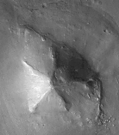
[/caption] The Pyramids on Mars are hills or mountains on the surface of Mars that, from a low resolution image, have near-perfect symmetry resembling that of the Egyptian pyramids. These formations are found in the Martian region known as Cydonia, an albedo feature that gained celebrity-like attention in the 1970s.
Some of the images captured of the Martian surface by the Viking Missions in the 70’s showed a formation that closely resembled a humanoid face. E.T. aficionados immediately interpreted this as a structure built by intelligent lifeforms like ours. More photographs of the region (Cydonia) revealed pyramid-like structures.
One of them, the D&M pyramid had a near-perfect symmetry. Since the pyramids were located near the “Face on Mars”, speculations regarding its alien origins gained more followers. According to advocates of the theory, the Face on Mars may have been constructed by inhabitants of the nearby city a.k.a. the Pyramids on Mars.
They even pointed out the peculiar smoothness of the wide region beside the Pyramids on Mars, which may have been a vast body of water such as an ocean. The proximity of the ‘city’ to a large body of water is typical of most inhabitants who would naturally want to be near a huge source of natural resources and a medium for travel.
This fascinating theory or story later on subsided when much higher resolution photos from later expeditions, one in April 5, 1998 and another in April 8, 2001, revealed the Face on Mars as nothing more than a mesa, an elevated piece of land with a flat top and steep sides. Mesas can be found in the southwestern region of the US.
You can also find them in South Africa, Arabia, India, Australia, and of course, Spain. The term ‘mesa’ is actually derived from the Spanish word that means ‘table’. Mesas look pretty much like giant tables rising above a surrounding plain.
The sharper images showed that the top of the mesa did not resemble a face at all. As for the Pyramids on Mars, such geological formations can be found here on Earth. They’re usually formed through the action of ice in glaciation or frost weathering.
Some good examples of such formations here on Earth are Switzerland’s Matterhorn, USA’s Mount Thielsen, Scotland’s Buachaille Etive Mòr, and Canada’s Mount Assiniboine.
We have some related articles here that may interest you:
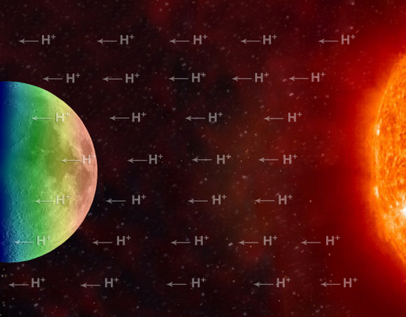
Schematic showing the stream of charged hydrogen ions carried from the Sun by the solar wind. One possible scenario to explain hydration of the lunar surface is that during the daytime, when the Moon is exposed to the solar wind, hydrogen ions liberate oxygen from lunar minerals to form OH and H2O, which are then weakly held to the surface. At high temperatures (red-yellow) more molecules are released than adsorbed. When the temperature decreases (green-blue) OH and H2O accumulate. [Image courtesy of University of Maryland/F. Merlin/McREL]
”]
Three different spacecraft have confirmed there is water on the Moon. It hasn’t been found in deep dark craters or hidden underground. Data indicate that water exists diffusely across the moon as hydroxyl or water molecules — or both — adhering to the surface in low concentrations. Additionally, there may be a water cycle in which the molecules are broken down and reformulated over a two week cycle, which is the length of a lunar day. This does not constitute ice sheets or frozen lakes: the amounts of water in a given location on the Moon aren’t much more than what is found in a desert here on Earth. But there’s more water on the Moon than originally thought.
The Moon was believed to extremely dry since the return of lunar samples from the Apollo and Luna programs. Many Apollo samples contain some trace water or minor hydrous minerals, but these have typically been attributed to terrestrial contamination since most of the boxes used to bring the Moon rocks to Earth leaked. This led the scientists to assume that the trace amounts of water they found came from Earth air that had entered the containers. The assumption remained that, outside of possible ice at the moon’s poles, there was no water on the moon.
Forty years later, an instrument on board the ill-fated Chandrayaan-1 spacecraft, the Moon Mineralogy Mapper (M cubed) found that infrared light was being absorbed near the lunar poles at wavelengths consistent with hydroxyl- and water-bearing materials.
M3 analyzes the way that light from the sun reflects off the lunar surface to understand what materials comprise the lunar soil. Light is reflected in different wavelengths off of different minerals, and specifically, the instrument detected wavelengths of reflected light that would indicate a chemical bond between hydrogen and oxygen. Given water’s well-known chemical symbol, H2O, which represents two hydrogen atoms bonded to one oxygen atom, this discovery was a source of great interest to the researchers.
The instrument can only see the very uppermost layers of the lunar soil – perhaps to a few centimeters below the surface. The scientists were looking for a signature of water in the craters near the poles, but found evidence for water instead on the sunlit portions of the moon. This was certainly unexpected and the science team from M3 looked and re-looked at their data for several months.
Confirmation came from a recent flyby of the re-purposed Deep Impact probe, on its way to rendezvous with another comet in 2010. In June of 2009, the spectrometer on board also showed strong evidence that water is ubiquitous over the surface of the moon.
Jessica Sunshine and colleagues with Deep Impact also found the presence of bound water or hydroxyl in trace amounts over much of the Moon’s surface. Their results suggest that the formation and retention of these molecules is an ongoing process on the lunar surface – and that solar wind could be responsible for forming them.
Still another spacecraft, the Cassini spacecraft while on its way to Saturn, also flew by the Moon in 1999. Roger Clark, a U.S. Geological Survey spectroscopist on the M3 team, reanalyzed archival data from Cassini, and that data as well agreed with the finding that water appears to be widespread across the lunar surface.
There are potentially two types of water on the moon: exogenic, meaning water from outside sources, such as comets striking the moon’s surface, and endogenic, meaning water that originates on the moon. The M3 research team, which includes Larry Taylor of the University of Tennessee, Knoxville, suspect that the water they’re seeing in the moon’s surface is endogenic.
But where did the water come from?
The team from M3 believe it may come from the solar wind.
As the sun undergoes nuclear fusion, it constantly emits a stream of particles, mostly protons, which are positively charged hydrogen atoms. On Earth, the atmosphere and magnetism prevent us from being bombarded by these protons, but the moon lacks that protection, meaning the oxygen-rich minerals and glasses on the surface of the moon are constantly pounded by hydrogen in the form of protons, moving at velocities of one-third the speed of light.
When those protons hit the lunar surface with enough force, suspects Taylor, they break apart oxygen bonds in soil materials, and where free oxygen and hydrogen are together, there’s a high chance that trace amounts of water will be formed. These traces are thought to be about a quart of water per ton of soil.
“The isotopes of oxygen that exist on the moon are the same as those that exist on Earth, so it was difficult if not impossible to tell the difference between water from the moon and water from Earth,” said Taylor. “Since the early soil samples only had trace amounts of water, it was easy to make the mistake of attributing it to contamination.”
Lead image caption: Schematic showing the stream of charged hydrogen ions carried from the Sun by the solar wind. One possible scenario to explain hydration of the lunar surface is that during the daytime, when the Moon is exposed to the solar wind, hydrogen ions liberate oxygen from lunar minerals to form OH and H2O, which are then weakly held to the surface. At high temperatures (red-yellow) more molecules are released than adsorbed. When the temperature decreases (green-blue) OH and H2O accumulate. Image courtesy of University of Maryland/F. Merlin/McREL
Here are some cool pictures of rivers taken by various spacecraft.
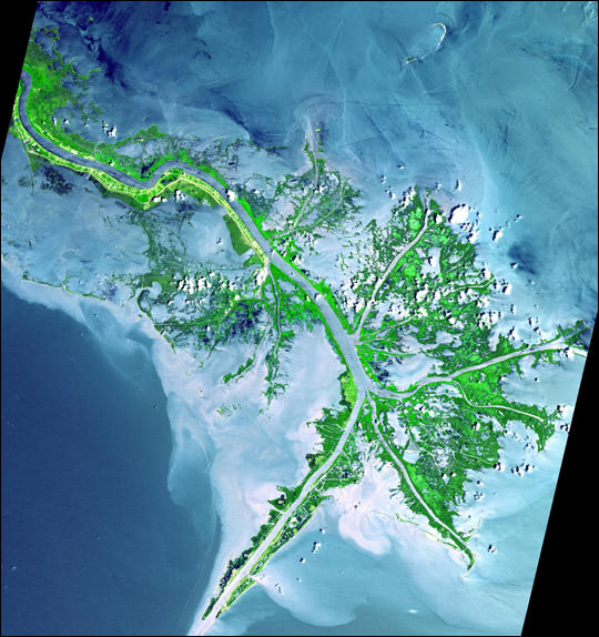
Here’s a picture of the Mississippi river delta. The image was captured by Advanced Spaceborne Thermal Emission and Reflection Radiometer (ASTER) aboard NASA’s Terra satellite.
Betsiboka River flooding
This is an image of flooding on the Betsiboka River in Madagascar. The flooding was created by Tropical Storm Eric, which swept through the region in early 2009. This photograph was taken by astronauts on board the International Space Station.
Colorado River Delta
People rely on the Colorado River so much that very little of it actually reaches the ocean. Instead, almost all of the water that flows through the river is used for irrigation along its route.
Ganges river delta. Image credit: NASA
This is a picture of the river delta for the Ganges. In fact, the Ganges combined with the Brahmaputra River make up the largest river delta in the world. The rivers flood from snow melt in the nearby Himalayas.
Niger River
This is a picture of the Niger River. It was captured by the ASTER instrument on board NASA’s Terra Earth Observation satellite.
[/caption]
A black dwarf is a white dwarf that has cooled down to the temperature of the cosmic microwave background, and so is invisible. Unlike red dwarfs, brown dwarfs, and white dwarfs, black dwarfs are entirely hypothetical.
Once a star has evolved to become a white dwarf, it no longer has an internal source of heat, and is shining only because it is still hot. Like something taken from the oven, left alone a white dwarf will cool down until it is the same temperature as its surroundings. Unlike tonight’s dinner, which cools by convection, conduction, and radiation, a white dwarf cools only by radiation.
Because it’s electron degeneracy pressure that stops it from collapsing to become a black hole, a white dwarf is a fantastic conductor of heat (in fact, the physics of Fermi gasses explains the conductivity of both white dwarfs and metals!). How fast a white dwarf cools is thus easy to work out … it depends on only its initial temperature, mass, and composition (most are carbon plus oxygen; some maybe predominantly oxygen, neon and magnesium; others helium). Oh, and as at least part of the core of a white dwarf may crystallize, the cooling curve will have a bit of a bump around then.
The universe is only 13.7 billion years old, so even a white dwarf formed 13 billion years ago (unlikely; the stars which become white dwarfs take a billion years, or so, to do so) it would still have a temperature of a few thousand degrees. The coolest white dwarf observed to date has a temperature of a little less than 3,000 K. A long way to go before it becomes a black dwarf.
Working out how long it would take for a white dwarf to cool to the temperature of the CMB is actually quite tricky. Why? Because there are lots of interesting effects that may be important, effects we cannot model yet. For example, a white dwarf will contain some dark matter, and at least some of that may decay, over timespans of quadrillions of years, generating heat. Perhaps diamonds are not forever (protons too may decay); more heat. And the CMB is getting cooler all the time too, as the universe continues to expand.
Anyway, if we say, arbitrarily, that at 5 K a white dwarf becomes a black dwarf, then it’ll take at least 10^15 years for one to form.
One more thing: no white dwarf is totally alone; some have binary companions, others may wander through a dust cloud … the infalling mass generates heat too, and if enough hydrogen builds up on the surface, it may go off like a hydrogen bomb (that’s what novae are!), warming the white dwarf quite a bit.
[/caption]
Want to find some cool Solar System coloring pages? Here are some links to resources we’ve been able to dig up from around the Internet.
Check out the offerings from Coloring Castle. I find it cool that they offer a version with Pluto, and then another without Pluto.
And one of the best resources on the internet for this kind of thing is Enchanted Learning. They’ve got a page just for Solar System coloring pages.
Windows on the Universe has coloring pages for all the planets in the Solar System. They even have an entire PDF book that you can print off with all the planets (including Pluto).
Coloring Fun has some more solar system pages for coloring.
[/caption]
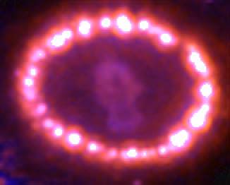
The first supernova in 1987 (that’s what the “A” means) was the brightest supernova in several centuries (and the first observed since the invention of the telescope), the first (and so far only) one to be detected by its neutrino emissions, and the only one in the LMC (Large Magellanic Cloud) observed directly.
Ian Shelton, then a research assistant with the University of Toronto, working at the university’s Las Campanas station, and Oscar Duhalde, a telescope operator at Las Campanas Observatory, were the first to spot it, on the night of 23/24 February 1987 (around midnight actually); over the next 24 hours several others also independently discovered it.
The IAU’s CBAT went wild! That’s the International Astronomical Union’s Central Bureau for Astronomical Telegrams, the clearing house for astronomers for breaking news. You can read the historic IAUC (C for Circular) 4416 here.
Once the discovery of SN 1987A became known, physicists examined the records from various neutrino detectors … and found three, independent, clear signals of a burst of neutrinos several hours before visual discovery, just as predicted by astrophysical models! Champagne flowed.
Not long afterwards, the star which blew up so spectacularly – the progenitor – was identified as Sanduleak -69° 202a, a blue supergiant. This was not what was expected for a Type II supernova (the models said red supergiants), but an explanation was quickly found (Sanduleak -69° 202a had a lower-than-modelled oxygen abundance, affecting the transparency of its outer envelope).
The iconic Hubble Space Telescope image (above) of SN 1987A shows the inner ring, where the debris from the explosion is colliding with matter expelled from the progenitor about 20,000 years ago; more from the Hubble here.
AAVSO (American Association of Variable Star Observers) has a nice write-up of SN 1987A.
[/caption]
“The square of the orbital period of a planet is proportional to the cube of the semi-major axis of its orbit” That’s Kepler’s third law. In other words, if you square the ‘year’ of each planet, and divide it by the cube of its distance to the Sun, you get the same number, for all planets.
(The other two are “the orbit of each planet is an ellipse with the Sun at a focus”, and “a line between a planet and the Sun sweeps out equal areas in equal times”.)
Copernicus, Kepler, and Newton dealt a one-two-three knockout blow to the idea – thousands of years old – that the Sun (and planets) moved around the Earth. Copernicus put the Sun at the center, Kepler modified Copernicus’ circular motions (and provided a simple, quantitative description of the actual motion), and Newton explained how it all worked (gravity).
Kepler worked out his three laws from detailed records of observations of the positions of the planets (known at the time, Mercury, Venus, Mars, Jupiter, and Saturn) – especially Mars – painstakingly compiled by Tycho Brahe.
Kepler’s third law (in fact, all three) works not only for the planets in our solar system, but also for the moons of all planets, dwarf planets and asteroids, satellites going round the Earth, etc. Well, not quite; if the secondary body – a planet, say – has a mass that’s a significant fraction of the primary one (the Sun, say), then the law needs a small tweak.
By showing how Kepler’s laws could be derived from his universal law of gravitation, Newton united heaven and earth, perhaps the greatest revolution in science (OK, Darwin’s revolution may be greater). Before Newton, the heavens were thought to work according to rules quite different from the ones which governed things on Earth.
NASA’s Imagine the Universe! has a neat demonstration of Kepler’s laws, and this PDF file (from the University of Tennessee Knoxville’s Maths Department) gives a simple derivation of Kepler’s laws, from Newton’s universal law of gravitation.
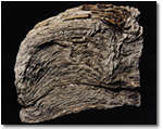
Fossil stromatolite, Barberton Mountains South Africa (2.5 billion years old)
[/caption]
How did life on Earth arise? Scientific efforts to answer that question are called abiogenesis. More formally, abiogenesis is a theory, or set of theories, concerning how life on Earth began (but excluding panspermia).
Note that while abiogenesis and evolution are related, they are distinct (evolution says nothing about how life began; abiogenesis says nothing about how life evolves).
Intensive study of the Earth’s rocks has turned up lots and lots of evidence that some kinds of prokaryotes lived happily on Earth about 3.5 billion years ago (and there’re also pointers to the existence of life on Earth in the oldest rocks). So, if life arose on Earth, it did so from the chemicals in the water, air, and rocks of the early Earth … and in no more than a few hundred million years.
Because there are no sedimentary rocks older than about 3.7 billion years (and no metamorphic ones older than about 3.9 billion years), and because the oldest such rocks already contain evidence that there was life on Earth then, testing abiogenesis theories must be done by means other than geological.
There is a long history of attempts to create various organic molecules – such as amino acids – from simple precursors such as carbon dioxide, ammonia, and water, in conditions which simulate those of the early Earth. Those of Miller and Urey, in 1953, are the most famous (and the first).
It turns out that it’s pretty easy to form many kinds of organic molecules, in a wide range of environments … so the focus of research today is on how life could arise from any particular brew. And the hard part is how reliable self-replication get going (if you can make some sort of primitive cell in a test tube, it isn’t a form of life if it can’t reproduce itself!). So far, it seems that RNA and DNA cannot have been involved (too hard to form and stay stable), but several simpler kinds of molecules may work.
Well, that’s one hard part; another is how can a stable bag of chemicals form? (There have been some exciting recent discoveries which may help answer at least part of this question).
A different approach – than reproduction – to finding the key to how life got started involves asking how metabolism arose; how can a bag of chemicals take in ‘food’, process it (to supply energy to all the other chemical processes going on in the bag), and get rid of the waste?
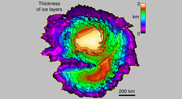
A radar-generated map of the thickness of the layered deposits. Image credit: NASA/JPL-Caltech/University of Rome/Southwest Research Institute/University of Arizona
[/caption]
A radar instrument on the Mars Reconnaissance Orbiter has essentially looked below the surface of the Red Planet’s north-polar ice cap, and found data to confirm theoretical models of Martian climate swings during the past few million years. The new, three-dimensional map using 358 radar observations provides a cross-sectional view of the north-polar layered deposits. “The radar has been giving us spectacular results,” said Jeffrey Plaut of JPL, a member of the science team for the Shallow Radar instrument. “We have mapped continuous underground layers in three dimensions across a vast area.”
Alignment of the layering patterns with the modeled climate cycles provides insight about how the layers accumulated. These ice-rich, layered deposits cover an area one-third larger than Texas and form a stack up to 2 kilometers (1.2 miles) thick atop a basal deposit with additional ice.
“Contrast in electrical properties between layers is what provides the reflectivity we observe with the radar,” said Nathaniel Putzig of Southwest Research Institute, Boulder, CO, who led the science team. “The pattern of reflectivity tells us about the pattern of material variations within the layers.”
Earlier radar observations indicated that the Martian north-polar layered deposits are mostly ice. Radar contrasts between different layers in the deposits are interpreted as differences in the concentration of rock material, in the form of dust, mixed with the ice. These deposits on Mars hold about one-third as much water as Earth’s Greenland ice sheet.
Their radar results show that high-reflectivity zones, with multiple contrasting layers, alternate with more-homogenous zones of lower reflectivity. Patterns of how these two types of zones alternate can be correlated to models of how changes in Mars’ tilt on its axis have produced changes in the planet’s climate in the past 4 million years or so, but only if some possibilities for how the layers form are ruled out.
“We’re not doing the climate modeling here; we are comparing others’ modeling results to what we observe with the radar, and using that comparison to constrain the possible explanations for how the layers form,” Putzig said.
The most recent 300,000 years of Martian history are a period of less dramatic swings in the planet’s tilt than during the preceding 600,000 years. Since the top zone of the north-polar layered deposits — the most recently deposited portion — is strongly radar-reflective, the researchers propose that such sections of high-contrast layering correspond to periods of relatively small swings in the planet’s tilt.
They also propose a mechanism for how those contrasting layers would form. The observed pattern does not fit well with an earlier interpretation that the dustier layers in those zones are formed during high-tilt periods when sunshine on the polar region sublimates some of the top layer’s ice and concentrates the dust left behind. Rather, it fits an alternative interpretation that the dustier layers are simply deposited during periods when the atmosphere is dustier.
The new radar mapping of the extent and depth of five stacked units in the north-polar layered deposits reveals that the geographical center of ice deposition probably shifted by 400 kilometers (250 miles) or more at least once during the past few million years.
The Italian Space Agency operates the Shallow Radar instrument.
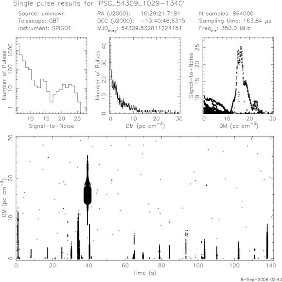
When Lucas Bolyard looked at the bottom plot, he noticed the thick, black blob left of the center. He saw that this signal was positioned on the graph where it indicated a non-zero "dispersion measure," or DM. Dispersion measure is used by astronomers as an indicator of cosmic distances. The non-zero DM value of this pulse is a clue that the signal came from space, not from Earth. The other blobs on the bottom of the graph are signals at a distance of zero-- that is from here on Earth. CREDIT: NRAO/AUI/NSF
[/caption]
A high-school student from West Virginia has discovered a new astronomical object, a strange type of neutron star called a rotating radio transient. Lucas Bolyard, a sophomore at South Harrison High School in Clarksburg, WV, made the discovery while participating in a project in which students are trained to search through data from the Robert C. Byrd Green Bank Telescope (GBT). Bolyard made the discovery in March, after he already had studied more than 2,000 data plots from the GBT and found nothing.
The project is the Pulsar Search Collaboratory (PSC), which allows students to do real scientific research by looking at data from the GBT, the largest radio telescope in the US. Lucas Bolyard CREDIT: NRAO/AUI/NSF
“Lucas is one of the most enthusiastic students involved in the project,” said Duncan Lorimer, astronomer from West Virginia University. “He’s one of these youngsters that never gives up, he’s very persistent and he has all the attributes that a scientist should have.”
Rotating radio transients are thought to be similar to pulsars, superdense neutron stars that are the corpses of massive stars that exploded as supernovae. Pulsars are known for their lighthouse-like beams of radio waves that sweep through space as the neutron star rotates, creating a pulse as the beam sweeps by a radio telescope. While pulsars emit these radio waves continuously, rotating radio transients emit only sporadically, one burst at a time, with as much as several hours between bursts. Because of this, they are difficult to discover and observe, with the first one only discovered in 2006.
“This neutron star is rotating very rapidly, so you have something the size of city with the mass of the sun, spinning incredibly rapidly,” said Lorimer “which also has an incredibly large magnetic field which is how we detect it with radio telescopes.”
“These objects are very interesting, both by themselves and for what they tell us about neutron stars and supernovae,” said Maura McLaughlin, also from WVU. “We don’t know what makes them different from pulsars — why they turn on and off. If we answer that question, it’s likely to tell us something new about the environments of pulsars and how their radio waves are generated.”
“They also tell us there are more neutron stars than we knew about before, and that means there are more supernova explosions. In fact, we now almost have more neutron stars than can be accounted for by the supernovae we can detect,” she added. Robert C. Byrd Green Bank Telescope CREDIT: NRAO/AUI/NSF
“I was home on a weekend and had nothing to do, so I decided to look at some more plots from the GBT,” Bolyard said. “I saw a plot with a pulse, but there was a lot of radio interference, too. The pulse almost got dismissed as interference,” he added.
Nonetheless, he reported it, and it went on a list of candidates for McLaughlin and Lorimer to re-examine, scheduling new observations of the region of sky from which the pulse came. Disappointingly, the follow-up observations showed nothing, indicating that the object was not a normal pulsar. However, the astronomers explained to Bolyard that his pulse still might have come from a rotating radio transient.
Confirmation didn’t come until July. Bolyard was at the NRAO’s Green Bank Observatory with fellow PSC students. The night before, the group had been observing with the GBT in the wee hours, and all were very tired. Then Lorimer showed Bolyard a new plot of his pulse, reprocessed from raw data, indicating that it is real, not interference, and that Bolyard is likely the discoverer of one of only about 30 rotating radio transients known.
Suddenly, Bolyard said, he wasn’t tired anymore. “That news made me full of energy,” he exclaimed. “My friends were really excited because they think I’m going to be famous!”
As of a year ago, Bolyard said he wouldn’t have thought of becoming astronomer, but this has given him second thoughts. “Making this discovery has made me very excited to get into a scientific field,” he said. “It’s a lot of hard work, but it’s worth it.”
The PSC, led by NRAO Education Officer Sue Ann Heatherly and Project Director Rachel Rosen, includes training for teachers and student leaders, and provides parcels of data from the GBT to student teams. The project involves teachers and students in helping astronomers analyze data from 1500 hours of observing with the GBT. The 120 terabytes of data were produced by 70,000 individual pointings of the giant, 17-million-pound telescope. Some 300 hours of the observing data were reserved for analysis by student teams.
The student teams use analysis software to reveal evidence of pulsars. Each portion of the data is analyzed by multiple teams. In addition to learning to use the analysis software, the student teams also must learn to recognize man-made radio interference that contaminates the data. The project will continue through 2011.
“The students get to actually look through data that has never been looked through before,” Rosen said. From the training, she added, “the students get a wonderful grasp of what they’re looking at, and they understand the science behind the plots that they’re looking at.”