Matt Williams is a space journalist and science communicator for Universe Today and Interesting Engineering. He's also a science fiction author, podcaster (Stories from Space), and Taekwon-Do instructor who lives on Vancouver Island with his wife and family.
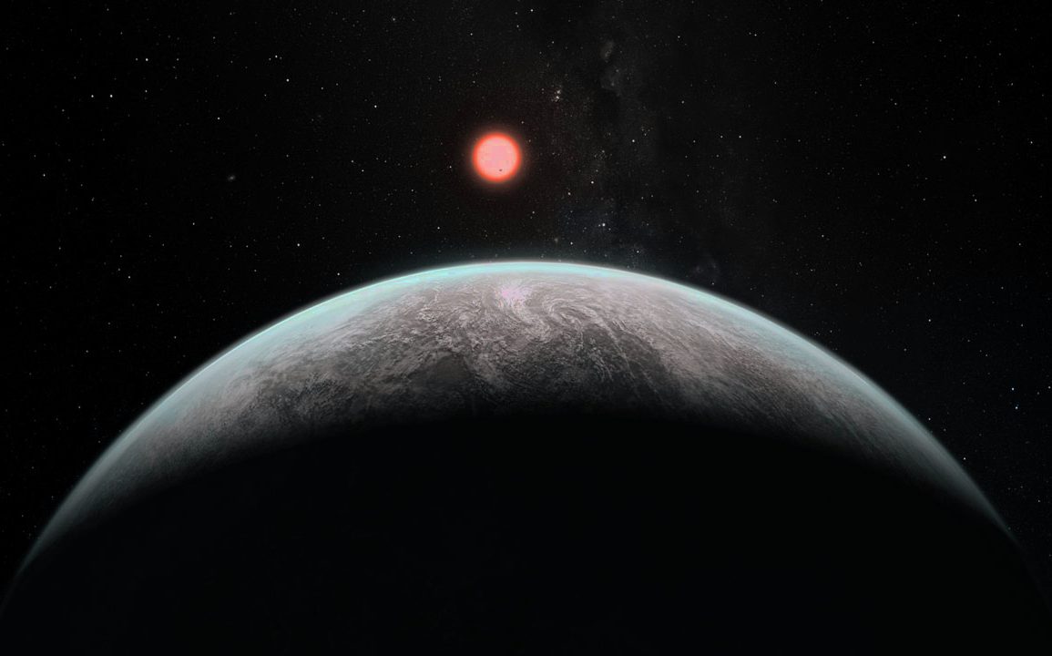
Artist’s impression of how an an Earth-like exoplanet might look. Credit: ESO.
The ongoing hunt for exoplanets has yielded some very interesting returns in recent years. All told, the Kepler mission has discovered more than 4000 candidates since it began its mission in March of 2009. Amidst the many “Super-Jupiters” and assorted gas giants (which account for the majority of Kepler’s discoveries) astronomers have been particularly interested in those exoplanets which resemble Earth.
And now, an international team of scientists has finished perusing the Kepler catalog in an effort to determine just how many of these planets are in fact “Earth-like”. Their study, titled “A Catalog of Kepler Habitable Zone Exoplanet Candidates” (which will be published soon in the AstrophysicalJournal), explains how the team discovered 216 planets that are both terrestrial and located within their parent star’s “habitable zone” (HZ).
The international team was made up of researchers from NASA, San Francisco State University, Arizona State University, Caltech, University of Hawaii-Manoa, the University of Bordeaux, Cornell University and the Harvard-Smithsonian Center for Astrophysics. Having spent the past three years looking over the more than 4000 entries, they have determined that 20 of the candidates are most like Earth (i.e. likely habitable).
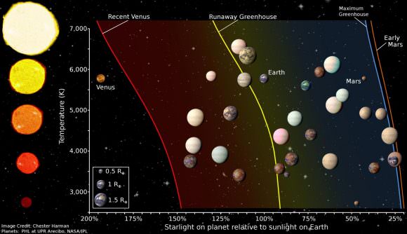
Figure showing the habitable zone for different types of stars, as well as the location of terrestrial size Kepler candidates. Credit: Chester Harman
As Stephen Kane, an associate professor of physics and astronomy at San Fransisco University and lead author of the study, explained in a recent statement:
“This is the complete catalog of all of the Kepler discoveries that are in the habitable zone of their host stars. That means we can focus in on the planets in this paper and perform follow-up studies to learn more about them, including if they are indeed habitable.”
In addition to isolating 216 terrestrial planets from the Kepler catalog, they also devised a system of four categories to determine which of these were most like Earth. These included “Recent Venus”, where conditions are like that of Venus (i.e. extremely hot); “Runaway Greenhouse”, where planets are undergoing serious heating; “Maximum Greenhouse”, where planets are within their star’s HZ; and “Recent Mars”, where conditions approximate those of Mars.
From this, they determined that of the Kepler candidates, 20 had radii less than twice that of Earth (i.e. on the smaller end of the Super-Earth category) and existed within their star’s HZ. In other words, of all the planets discovered in our local Universe, they were able to isolate those where liquid water can exist on the surface, and the gravity would likely be comparable to Earth’s and not crushing!
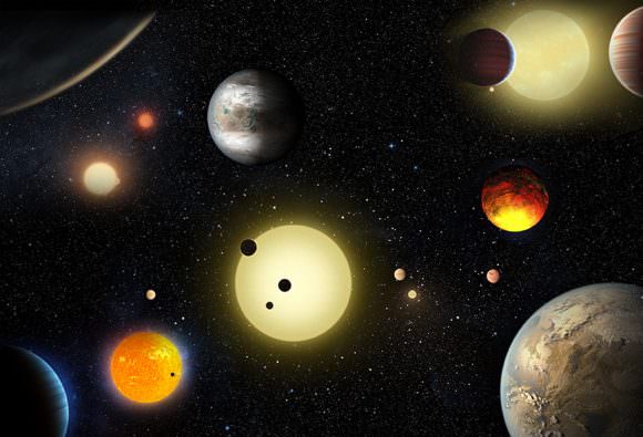
Earlier today, NASA announced that Kepler had confirmed the existence of 1,284 new exoplanets, the most announced at any given time. Credit: NASA
This is certainly exciting news, since one of the most important aspects of exoplanet hunting has been finding worlds that could support life. Naturally, it might sound a bit anthropocentric or naive to assume that planets which have similar conditions to our own would be the most likely places for it to emerge. But this is what is known as the “low-hanging fruit” approach, where scientists seek out conditions which they know can lead to life.
“There are a lot of planetary candidates out there, and there is a limited amount of telescope time in which we can study them,” said Kane. “This study is a really big milestone toward answering the key questions of how common is life in the universe and how common are planets like the Earth.”
Professor Kane is renowned for being one of the world’s leading “planet-hunters”. In addition to discovering several hundred exoplanets (using data obtained by the Kepler mission) he is also a contributor to two upcoming satellite missions – the NASA Transiting Exoplanet Survey Satellite (TESS) and the European Space Agency’s Characterizing ExOPLanet Satellite (CHEOPS).
These next-generation exoplanet hunters will pick up where Kepler left off, and are likely to benefit greatly from this recent study.
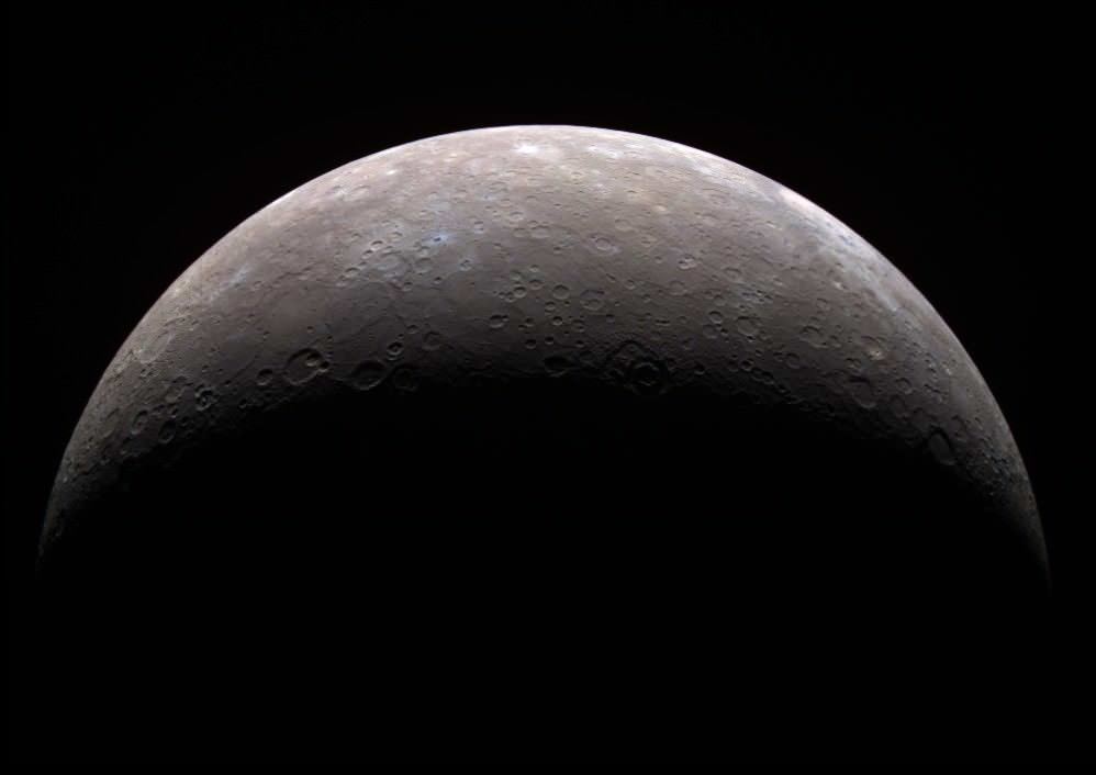
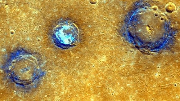
Planet Mercury as seen from the MESSENGER spacecraft in 2008. Credit: NASA/JPL
Welcome back to the first in our series on Settling the Solar System! First up, we take a look at that hot, hellish place located closest to the Sun – the planet Mercury!
Humanity has long dreamed of establishing itself on other worlds, even before we started going into space. We’ve talked about colonizing the Moon, Mars, and even establishing ourselves on exoplanets in distant star systems. But what about the other planets in our own backyard? When it comes to the Solar System, there is a lot of potential real estate out there that we don’t really consider.
Well, consider Mercury. While most people wouldn’t suspect it, the closest planet to our Sun is actually a potential candidate for settlement. Whereas it experiences extremes in temperature – gravitating between heat that could instantly cook a human being to cold that could flash-freeze flesh in seconds – it actually has potential as a starter colony.
Examples in Fiction:
The idea of colonizing Mercury has been explored by science fiction writers for almost a century. However, it has only been since the mid-20th century that colonization has been dealt with in a scientific fashion. Some of the earliest known examples of this include the short stories of Leigh Brackett and Isaac Asimov during the 1940s and 50s.
In the former’s work, Mercury is a tidally-locked planet (which was what astronomers believed at the time) that has a “Twilight Belt” characterized by extremes in heat, cold, and solar storms. Some of Asimov’s early work included short stories where a similarly tidally-locked Mercury was the setting, or characters came from a colony located on the planet.
Mercury, as imaged by the MESSENGER spacecraft, revealing parts of the never seen by human eyes. Credit: NASA/Johns Hopkins University Applied Physics Laboratory/Carnegie Institution of Washington
These included “Runaround” (written in 1942, and later included in I, Robot), which centers on a robot that is specifically designed to cope with the intense radiation of Mercury. In Asimov’s murder-mystery story “The Dying Night” (1956) – in which the three suspects hail from Mercury, the Moon, and Ceres – the conditions of each location are key to finding out who the murderer is.
In 1946, Ray Bradbury published “Frost and Fire”, a short story that takes place on a planet described as being next to the sun. The conditions on this world allude to Mercury, where the days are extremely hot, the nights extremely cold, and humans live for only eight days. Arthur C. Clarke’s Islands in the Sky (1952) contains a description of a creature that lives on what was believed at the time to be Mercury’s permanently dark side and occasionally visits the twilight region.
In his later novel, Rendezvous with Rama (1973), Clarke describes a colonized Solar System which includes the Hermians, a toughened branch of humanity that lives on Mercury and thrives off the export of metals and energy. The same setting and planetary identities are used in his 1976 novel Imperial Earth.
In Kurt Vonnegut’s novel The Sirens of Titan (1959), a section of the story is set in caves located on the dark side of the planet. Larry Niven’s short story “The Coldest Place” (1964) teases the reader by presenting a world that is said to be the coldest location in the Solar System, only to reveal that it is the dark side of Mercury (and not Pluto, as is generally assumed).
“Lava Falls on Mercury” (by Ken Fagg) for If magazine, June 1954. Credit: Public Domain
Mercury also serves as a location in many of Kim Stanley Robinson’s novels and short stories. These include The Memory of Whiteness (1985), Blue Mars (1996), and 2312 (2012), in which Mercury is the home to a vast city called Terminator. To avoid the harmful radiation and heat, the city rolls around the planet’s equator on tracks, keeping pace with the planet’s rotation so that it stays ahead of the Sun.
In 2005, Ben Bova published Mercury (part of his Grand Tour series) that deals with the exploration of Mercury and colonizing it for the sake of harnessing solar energy. Charles Stross’ 2008 novel Saturn’s Children involves a similar concept to Robinson’s 2312, where a city called Terminator traverses the surface on rails, keeping pace with the planet’s rotation.
Proposed Methods:
A number of possibilities exist for a colony on Mercury, owing to the nature of its rotation, orbit, composition, and geological history. For example, Mercury’s slow rotational period means that one side of the planet is facing towards the Sun for extended periods of time – reaching temperatures highs of up to 427 °C (800 °F) – while the side facing away experiences extreme cold (-193 °C; -315 °F).
In addition, the planet’s rapid orbital period of 88 days, combined with its sidereal rotation period of 58.6 days, means that it takes roughly 176 Earth days for the Sun to return to the same place in the sky (i.e. a solar day). Essentially, this means that a single day on Mercury lasts as long as two of its years. So if a city were placed on the night-side, and had tracks wheels so it could keep moving to stay ahead of the Sun, people could live without fear of burning up.
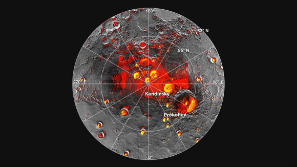
Images of Mercury’s northern polar region, provided by MESSENGER. Credit: NASA/JPL
In addition, Mercury’s very low axial tilt (0.034°) means that its polar regions are permanently shaded and cold enough to contain water ice. In the northern region, a number of craters were observed by NASA’s MESSENGER probe in 2012 which confirmed the existence of water ice and organic molecules. Scientists believe that Mercury’s southern pole may also have ice, and claim that an estimated 100 billion to 1 trillion tons of water ice could exist at both poles, which could be up to 20 meters thick in places.
In these regions, a colony could be built using a process called “paraterraforming” – a concept invented by British mathematician Richard Taylor in 1992. In a paper titled “Paraterraforming – The Worldhouse Concept”, Taylor described how a pressurized enclosure could be placed over the usable area of a planet to create a self-contained atmosphere. Over time, the ecology inside this dome could be altered to meet human needs.
In the case of Mercury, this would include pumping in a breathable atmosphere, and then melting the ice to create water vapor and natural irrigation. Eventually, the region inside the dome would become a livable habitat, complete with its own water cycle and carbon cycle. Alternately, the water could be evaporated, and oxygen gas created by subjecting it to solar radiation (a process known as photolysis).
Another possibility would be to build underground. For years, NASA has been toying with the idea of building colonies in stable, underground lava tubes that are known to exist on the Moon. And geological data obtained by the MESSENGER probe during flybys it conducted between 2008 and 2012 led to speculation that stable lava tubes might exist on Mercury as well.
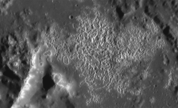
A previous MESSENGER image of hollows inside Tyagaraja crater. Credit: NASA/Johns Hopkins University Applied Physics Laboratory/Carnegie Institution of Washington
This includes information obtained during the probe’s 2009 flyby of Mercury, which revealed that the planet was a lot more geologically active in the past than previously thought. In addition, MESSENGER began spotting strange Swiss cheese-like features on the surface in 2011. These holes, which are known as “hollows”, could be an indication that underground tubes exist on Mercury as well.
Colonies built inside stable lava tubes would be naturally shielded to cosmic and solar radiation, extremes in temperature, and could be pressurized to create breathable atmospheres. In addition, at this depth, Mercury experiences far less in the way of temperature variations and would be warm enough to be habitable.
Potential Benefits:
At a glance, Mercury looks similar to the Earth’s Moon, so settling it would rely on many of the same strategies for establishing a moon base. It also has abundant minerals to offer, which could help move humanity towards a post-scarcity economy. Like Earth, it is a terrestrial planet, which means it is made up of silicate rocks and metals that are differentiated between an iron core and silicate crust and mantle.
However, Mercury is composed of 70% metals whereas’ Earth’s composition is 40% metal. What’s more, Mercury has a particular large core of iron and nickel, and which accounts for 42% of its volume. By comparison, Earth’s core accounts for only 17% of its volume. As a result, if Mercury were to be mined, enough minerals could be produced to last humanity indefinitely.
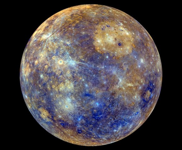
The different colors in this MESSENGER image of Mercury indicate the planet’s chemical, mineralogical, and physical differences. Credit: NASA/Johns Hopkins University Applied Physics Laboratory/Carnegie Institution of Washington.
Its proximity to the Sun also means that it could harness a tremendous amount of energy. This could be gathered by orbital solar arrays, which would be able to harness energy constantly and beam it to the surface. This energy could then be beamed to other planets in the Solar System using a series of transfer stations positioned at Lagrange Points.
Also, there’s the matter of Mercury’s gravity, which is 38% percent of Earth’s gravity. This is over twice what the Moon experiences, which means colonists would have an easier time adjusting to it. At the same time, it is also low enough to present benefits as far as exporting minerals is concerned, since ships departing from the surface would need less energy to achieve escape velocity.
Lastly, there is the distance to Mercury itself. At an average distance of about 93 million km (58 million mi), Mercury ranges between being 77.3 million km (48 million mi) to 222 million km (138 million mi) away from the Earth. This puts it a lot closer than other possible resource-rich areas like the Asteroid Belt (329 – 478 million km distant), Jupiter and its system of moons (628.7 – 928 million km), or Saturn’s (1.2 – 1.67 billion km).
Also, Mercury achieves inferior conjunction – the point where it is at its closest point to Earth – every 116 days, which is significantly shorter than either Venus’ or Mars’. Basically, missions destined for Mercury could launch almost every four months, whereas launch windows to Venus and Mars would have to take place every 1.6 years and 26 months, respectively.
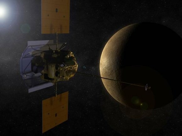
The MESSENGER spacecraft has been in orbit around Mercury since March 2011 – but its days are numbered. Credit: NASA/JHUAPL/Carnegie Institution of Washington
In terms of travel time, several missions have been mounted to Mercury that can give us a ballpark estimate of how long it might take. For instance, the first spacecraft to travel to Mercury, NASA’s Mariner 10 spacecraft (which launched in 1973), took about 147 days to get there.
More recently, NASA’s MESSENGER spacecraft launched on August 3rd, 2004 to study Mercury in orbit, and made its first flyby on January 14th, 2008. That’s a total of 1,260 days to get from Earth to Mercury. The extended travel time was due to engineers seeking to place the probe in orbit around the planet, so it needed to proceed at a slower velocity.
Challenges:
Of course, a colony on Mercury would still be a huge challenge, both economically and technologically. The cost of establishing a colony anywhere on the planet would be tremendous and would require abundant materials to be shipped from Earth, or mined on site. Either way, such an operation would require a large fleet of spaceships capable of making the journey in a respectable amount of time.
Such a fleet does not yet exist, and the cost of developing it (and the associated infrastructure for getting all the necessary resources and supplies to Mercury) would be tremendous. Relying on robots and in-situ resource utilization (ISRU) would certainly cut costs and reduce the amount of materials that would need to be shipped. But these robots and their operations would need to be shielded from radiation and solar flares until they got the job done.
Enhanced-color image of Munch, Sander, and Poe craters amid volcanic plains (orange) near Caloris Basin. Credit: NASA/Johns Hopkins University Applied Physics Laboratory/Carnegie Institution of Washington
Basically, the situation is like trying to establish a shelter in the middle of a thunderstorm. Once it is complete, you can take shelter. But in the meantime, you’re likely to get wet and dirty! And even once the colony was complete, the colonists themselves would have to deal with the ever-present hazards of radiation exposure, decompression, and extremes in heat and cold.
As such, if a colony was established on Mercury, it would be heavily dependent on its technology (which would have to be rather advanced). Also, until such time as the colony became self-sufficient, those living there would be dependent on supply shipments that would have to come regularly from Earth (again, shipping costs!)
Still, once the necessary technology was developed, and we could figure out a cost-effective way to create one or more settlements and ship to Mercury, we could look forward to having a colony that could provide us with limitless energy and minerals. And we would have a group of human neighbors known as Hermians!
As with everything else pertaining to colonization and terraforming, once we’ve established that it is in fact possible, the only remaining question is “how much are we willing to spend?”
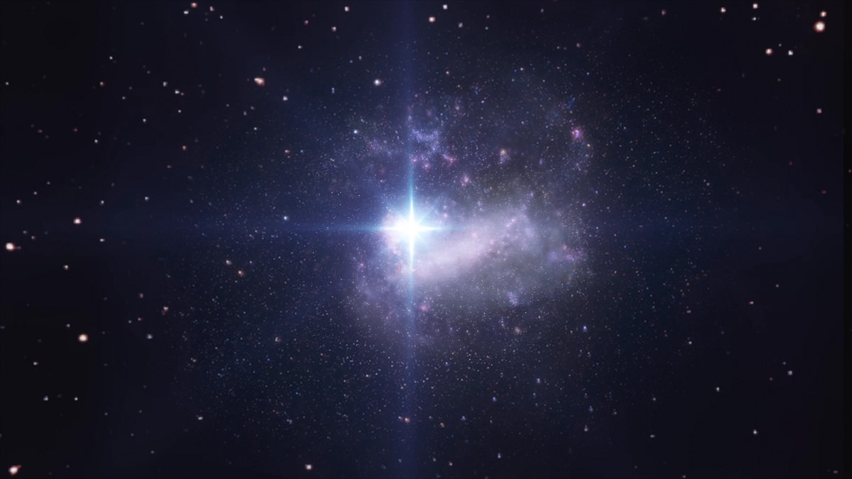
Artist’s impression of the supernova flare seen in the Large Magellanic Cloud on February 23rd, 1987. Credit: CAASTRO / Mats Björklund (Magipics).
Thirty years ago, a star that went by the designation of SN 1987A collapsed spectacularly, creating a supernova that was visible from Earth. This was the largest supernova to be visible to the naked eye since Kepler’s Supernova in 1604. Today, this supernova remnant (which is located approximately 168,000 light-years away) is being used by astronomers in the Australian Outback to help refine our understanding of stellar explosions.
Led by a student from the University of Sydney, this international research team is observing the remnant at the lowest-ever radio frequencies. Previously, astronomers knew much about the star’s immediate past by studying the effect the star’s collapse had on the neighboring Large Magellanic Cloud. But by detecting the star’s faintest hisses of radio static, the team was able to observe a great deal more of its history.
The team’s findings, which were published yesterday in the journal Monthly Notices of the Royal Astronomical Society, detail how the astronomers were able to look millions of years farther back in time. Prior to this, astronomers could only observe a tiny fraction of the star’s life cycle before it exploded – 20,000 years (or 0.1%) of its multi-million year life span.
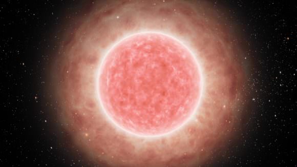
Artist’s impression of the star in its multi-million year long and previously unobservable phase as a large, red supergiant. Credit: CAASTRO / Mats Björklund (Magipics)
As such, they were only able to see the star when it was in its final, blue supergiant phase. But with the help of the Murchison Widefield Array (MWA) – a low-frequency radio telescope located at the Murchison Radio-astronomy Observatory (MRO) in the West Australian desert – the radio astronomers were able to see all the way back to when the star was still in its long-lasting red supergiant phase.
In so doing, they were able to observe some interesting things about how this star behaved leading up to the final phase in its life. For instance, they found that SN 1987A lost its matter at a slower rate during its red supergiant phase than was previously assumed. They also observed that it generated slower than expected winds during this period, which pushed into its surrounding environment.
Joseph Callingham, a PhD candidate with the University of Sydney and the ARC Center of Excellence for All-Sky Astrophysics (CAASTRO), is the leader of this research effort. As he stated in a recent RAS press release:
“Just like excavating and studying ancient ruins that teach us about the life of a past civilization, my colleagues and I have used low-frequency radio observations as a window into the star’s life. Our new data improves our knowledge of the composition of space in the region of SN 1987A; we can now go back to our simulations and tweak them, to better reconstruct the physics of supernova explosions.”
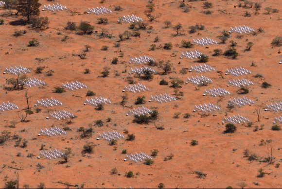
Aerial photograph of the core region of the MWA telescope. Credit: mwatelescope.org
The key to finding this new information was the quiet and (some would say) temperamental conditions that the MWA requires to do its thing. Like all radio telescopes, the MWA is located in a remote area to avoid interference from local radio sources, not to mention a dry and elevated area to avoid interference from atmospheric water vapor.
As Professor Gaensler – the former CAASTRO Director and the supervisor of the project – explained, such methods allow for impressive new views of the Universe. “Nobody knew what was happening at low radio frequencies,” he said, “because the signals from our own earthbound FM radio drown out the faint signals from space. Now, by studying the strength of the radio signal, astronomers for the first time can calculate how dense the surrounding gas is, and thus understand the environment of the star before it died.”
These findings will likely help astronomers to understand the life cycle of stars better, which will come in handy when trying to determine what our Sun has in store for us down the road. Further applications will include the hunt for extra-terrestrial life, with astronomers being able to make more accurate estimates on how stellar evolution could effect the odds of life forming in different star systems.
In addition to being home to the MWA, the Murchison Radio-astronomy Observatory (MRO) is also the planned site of the future Square Kilometer Array (SKA). The MWA is one of three telescopes – along with the South African MeerKAT array and the Australian SKA Pathfinder (ASKAP) array – that are designated as a Precursor for the SKA.
Artist's impression of an exoplanet orbiting a low-mass star. Credit: ESO/L. Calçada
The Fermi Paradox essentially states that given the age of the Universe, and the sheer number of stars in it, there really ought to be evidence of intelligent life out there. This argument is based in part on the fact that there is a large gap between the age of the Universe (13.8 billion years) and the age of our Solar System (4.5 billion years ago). Surely, in that intervening 9.3 billion years, life has had plenty of time to evolve in other star system!
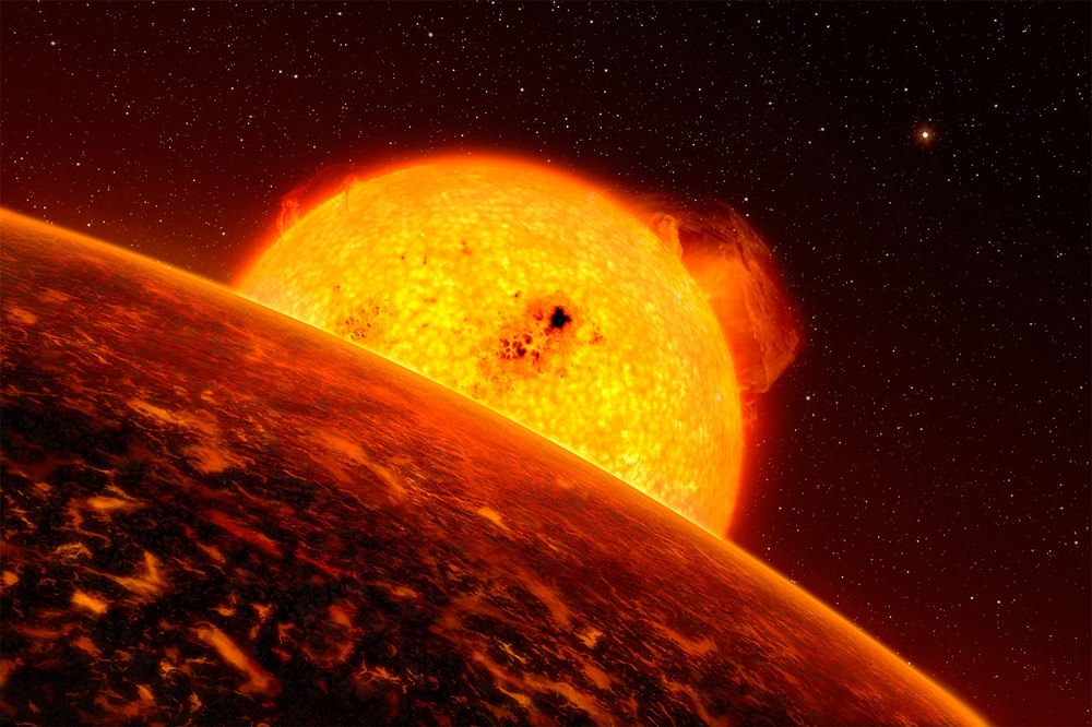
Artists concept for sending SpaceX Red Dragon spacecraft to land propulsively on Mars as early as 2020. Credit: SpaceX
Ever since Musk founded SpaceX is 2002, with the intention of eventually colonizing Mars, every move he has made has been the subject of attention. And for the past two years, a great deal of this attention has been focused specifically on the development of the Falcon Heavy rocket and the Dragon 2 capsule – the components with which Musk hopes to mount a lander mission to Mars in 2018.
Among other things, there is much speculation about how much this is going to cost. Given that one of SpaceX’s guiding principles is making space exploration cost-effective, just how much money is Musk hoping to spend on this important step towards a crewed mission? As it turns out, NASA produced some estimates at a recent meeting, which indicated that SpaceX is spending over $300 million on its proposed Mars mission.
These estimates were given during a NASA Advisory Council meeting, which took place in Cleveland on July 26th between members of the technology committee. During the course of the meeting, James L. Reuter – the Deputy Associate Administrator for Programs at NASA’s Space Technology Mission Directorate – provided an overview of NASA’s agreement with SpaceX, which was signed in December of 2014 and updated this past April.
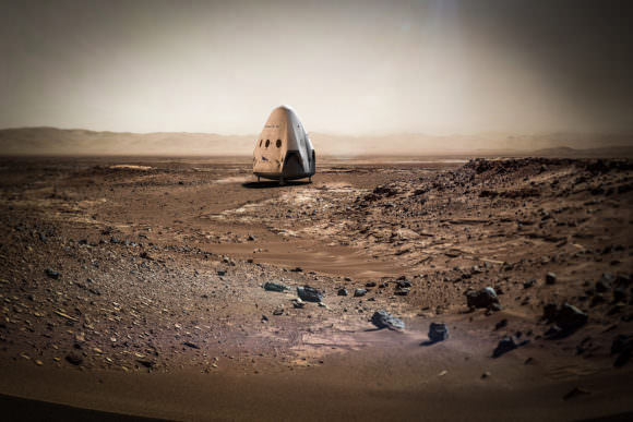
Artists concept for sending SpaceX Red Dragon spacecraft to land propulsively on Mars as early as 2018. Credit: SpaceX
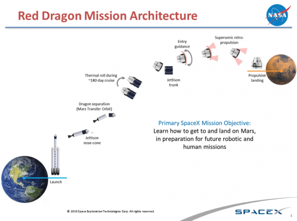
In accordance with this agreement, NASA will be providing support for the company’s plan to send an uncrewed Dragon 2 capsule (named “Red Dragon”) to Mars by May of 2018. Intrinsic to this mission is the plan to conduct a propulsive landing on Mars, which would test the Dragon 2‘s SuperDraco Descent Landing capability. Another key feature of this mission will involve using the Falcon Heavy to deploy the capsule.
The terms of this agreement do not involve the transfer of funds, but entails active collaboration that would be to the benefit parties. As Reuters indicated in his presentation, which NASA’s Office of Communications shared with Universe Today via email (and will be available on the STMD’s NASA page soon):
“Building on an existing no-funds-exchanged collaboration with SpaceX, NASA is providing technical support for the firm’s plan to attempt to land an uncrewed Dragon 2 spacecraft on Mars. This collaboration could provide valuable entry, descent and landing (EDL) data to NASA for our journey to Mars, while providing support to American industry. We have similar agreements with dozens of U.S. commercial, government, and non-profit partners.”
Further to this agreement is NASA’s commitment to a budget of $32 million over the next four years, the timetable of which were partially-illustrated in the presentation: “NASA will contribute existing agency resources already dedicated to [Entry, Descent, Landing] work, with an estimated value of approximately $32M over four years with approximately $6M in [Fiscal Year] 2016.”
According to Article 21 of the Space Act Agreement between NASA and SpaceX, this will include providing SpaceX with: “Deep space communications and telemetry; Deep space navigation and trajectory design; Entry, descent and landing system analysis and engineering support; Mars entry aerodynamic and aerothermal database development; General interplanetary mission advice and hardware consultation; and planetary protection consultation and advice.”
For their part, SpaceX has not yet disclosed how much their Martian mission plan will cost. But according to Jeff Foust of SpaceNews, Reuter provided a basic estimate of about $300 million based on a 10 to 1 assessment of NASA’s own financial commitment: “They did talk to us about a 10-to-1 arrangement in terms of cost: theirs 10, ours 1,” said Reuter. “I think that’s in the ballpark.”
As for why NASA has chosen to help SpaceX make this mission happen, this was also spelled out in the course of the meeting. According to Reuter’s presentation: “NASA conducted a fairly high-level technical feasibility assessment and determined there is a reasonable likelihood of mission success that would be enhanced with the addition of NASA’s technical expertise.”
Such a mission would provide NASA with valuable landing data, which would prove very useful when mounting its crewed mission in the 2030s. Other items discussed included NASA-SpaceX collaborative activities for the remainder of 2016 – which involved a “[f]ocus on system design, based heavily on Dragon 2 version used for ISS crew and cargo transportation”.
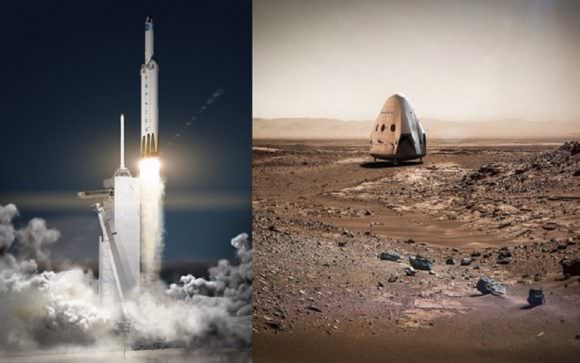
Artistic concepts of the Falcon Heavy rocket (left) and the Dragon capsule deployed on the surface of Mars (right). Credit: SpaceX
It was also made clear that the Falcon Heavy, which SpaceX is close to completing, will serve as the launch vehicle. SpaceX intends to conduct its first flight test (Falcon Heavy Demo Flight 1) of the heavy-lifter in December of 2016. Three more test flights are scheduled to take place between 2017 and the launch of the Mars lander mission, which is still scheduled for May of 2018.
In addition to helping NASA prepare for its mission to the Red Planet, SpaceX’s progress with both the Falcon Heavy and Dragon 2 are also crucial to Musk’s long-term plan for a crewed mission to Mars – the architecture of which has yet to be announced. They are also extremely important in the development of the Mars Colonial Transporter, which Musk plans to use to create a permanent settlement on Mars.
And while $300 million is just a ballpark estimate at this juncture, it is clear that SpaceX will have to commit considerable resources to the enterprise. What’s more, people must keep in mind that this would be merely the first in a series of major commitments that the company will have to make in order to mount a crewed mission by 2024, to say nothing of building a Martian colony!
In the meantime, be sure to check out this animation of the Crew Dragon in flight:
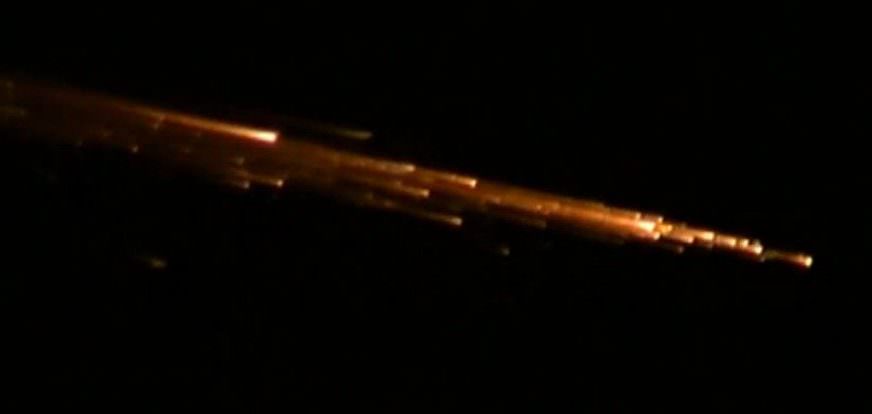
Astronomers have confirmed that the fiery debris spotted over the south-western US this week was a Chinese rocket. Credit: NBC
Seeing a fireball erupt in the sky is not an unusual occurrence. Especially during late July, when the Delta Aquirid meteor shower is so near to peaking. At times like this, dozens of fiery objects can be observed streaking across the atmosphere. But on this occasion, the light show that was spotted over Las Vegas earlier this week had a stranger cause.
The fireball appeared on Wednesday July 27th, at around 9:30 p.m. (Pacific Time), and could be seen from California to Utah. News and videos of the fiery apparition were quickly posted on social media, where astronomers began to notice something odd. And as it turned out, it was NOT the result of a meteor shower, but was in fact was the second stage of a rocket hitting the atmosphere, courtesy of the Chinese National Space Agency.
Such was the conclusion of Phil Plait, an astronomer and writer for Slate. After seeing a video shot of the display, he took to Twitter to question the explanation that it was the result of the Delta Aquirids. Based on his observations, he asserted that the event was actually the result of space debris burning up in the atmosphere.
His posts encouraged Jonathan McDowell, an astronomer at the Harvard-Smithsonian Center for Astrophysics, to do some checking. After looking into the matter, McDowell determined that the cause was a spent stage of a Chinese rocket falling back to Earth. As he posted on Twitter:
“Observation reports from Utah indicate the second stage from the first Chang Zheng 7 rocket, launched Jun 25, reentered at 0440 UTC.”
The Chang Zheng 7 is the latest in a line of Chinese rockets. It’s name translates to “Long March”, in honor of Mao’s forces marching into China’s interior during the Second Sino-Japanese War (1937-1945). A liquid-fueled carrier rocket designed to handle medium to heavy payloads, this rocket was developed to replace the Chinese Space Agency’s Long March 2F crew-rated launch vehicle.
This rocket is expected to play a critical role in creation of the Chinese Space Station, and will serve as the launch vehicle for the Tianzhou robotic cargo spacecraft in the meantime. Monday, June 25th was the inaugural launch of the rocket, and after the second stage was spent, it re-entered the Earth’s atmosphere at 04:36 UTC (9:36 p.m. Pacific Time) on Wednesday.
The 2nd stage then began to burn up as it moved across the sky from southwest to northeast, moving at speeds of 20,000 km/h (12,427 mph). It eventually disintegrated after becoming visible all across the south-western US, burning up at an altitude of about 100 km (62.13 mi). At this point, observers reported hearing a large boom, and many were fortunate enough to get the whole thing on video (as you can see from the ones included here).
While discarded space vehicles burn up in the atmosphere all the time, this was one of those rare occasions when the object happened to weight 6 metric tons (6.6 short tons)! We’re just fortunate that space launches are so rigorously planned so as to prevent them from causing accidents and extensive property damage, unlike certain meteorites that show up uninvited (looking at you Chelyabinsk meteor!)
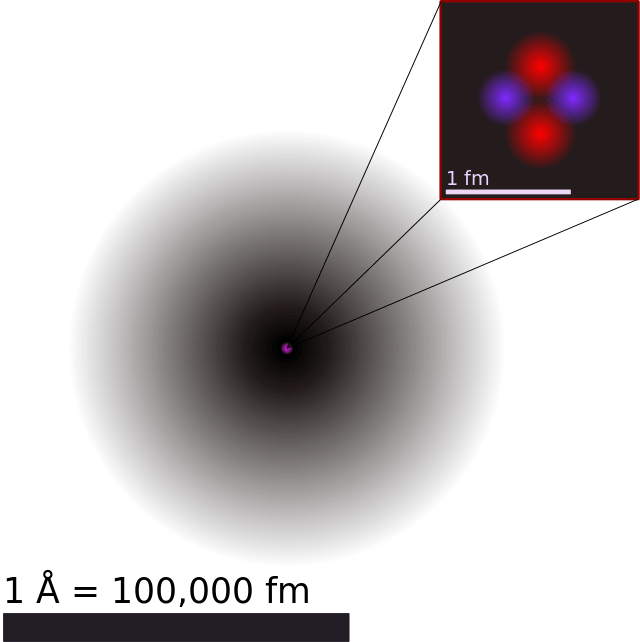
A depiction of the atomic structure of the helium atom. Credit: Creative Commons
Atomic theory has come a long way over the past few thousand years. Beginning in the 5th century BCE with Democritus‘ theory of indivisible “corpuscles” that interact with each other mechanically, then moving onto Dalton’s atomic model in the 18th century, and then maturing in the 20th century with the discovery of subatomic particles and quantum theory, the journey of discovery has been long and winding.
Arguably, one of the most important milestones along the way has been Bohr’ atomic model, which is sometimes referred to as the Rutherford-Bohr atomic model. Proposed by Danish physicist Niels Bohr in 1913, this model depicts the atom as a small, positively charged nucleus surrounded by electrons that travel in circular orbits (defined by their energy levels) around the center.
Atomic Theory to the 19th Century:
The earliest known examples of atomic theory come from ancient Greece and India, where philosophers such as Democritus postulated that all matter was composed of tiny, indivisible and indestructible units. The term “atom” was coined in ancient Greece and gave rise to the school of thought known as “atomism”. However, this theory was more of a philosophical concept than a scientific one.
Various atoms and molecules as depicted in John Dalton’s A New System of Chemical Philosophy (1808). Credit: Public Domain
It was not until the 19th century that the theory of atoms became articulated as a scientific matter, with the first evidence-based experiments being conducted. For example, in the early 1800’s, English scientist John Dalton used the concept of the atom to explain why chemical elements reacted in certain observable and predictable ways. Through a series of experiments involving gases, Dalton went on to develop what is known as Dalton’s Atomic Theory.
This theory expanded on the laws of conversation of mass and definite proportions and came down to five premises: elements, in their purest state, consist of particles called atoms; atoms of a specific element are all the same, down to the very last atom; atoms of different elements can be told apart by their atomic weights; atoms of elements unite to form chemical compounds; atoms can neither be created or destroyed in chemical reaction, only the grouping ever changes.
Discovery of the Electron:
By the late 19th century, scientists also began to theorize that the atom was made up of more than one fundamental unit. However, most scientists ventured that this unit would be the size of the smallest known atom – hydrogen. By the end of the 19th century, this would change drastically, thanks to research conducted by scientists like Sir Joseph John Thomson.
Through a series of experiments using cathode ray tubes (known as the Crookes’ Tube), Thomson observed that cathode rays could be deflected by electric and magnetic fields. He concluded that rather than being composed of light, they were made up of negatively charged particles that were 1ooo times smaller and 1800 times lighter than hydrogen.
The Plum Pudding model of the atom proposed by J.J. Thomson. Credit: britannica.com
This effectively disproved the notion that the hydrogen atom was the smallest unit of matter, and Thompson went further to suggest that atoms were divisible. To explain the overall charge of the atom, which consisted of both positive and negative charges, Thompson proposed a model whereby the negatively charged “corpuscles” were distributed in a uniform sea of positive charge – known as the Plum Pudding Model.
These corpuscles would later be named “electrons”, based on the theoretical particle predicted by Anglo-Irish physicist George Johnstone Stoney in 1874. And from this, the Plum Pudding Model was born, so named because it closely resembled the English desert that consists of plum cake and raisins. The concept was introduced to the world in the March 1904 edition of the UK’sPhilosophical Magazine, to wide acclaim.
The Rutherford Model:
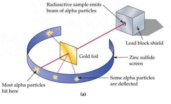
Subsequent experiments revealed a number of scientific problems with the Plum Pudding model. For starters, there was the problem of demonstrating that the atom possessed a uniform positive background charge, which came to be known as the “Thomson Problem”. Five years later, the model would be disproved by Hans Geiger and Ernest Marsden, who conducted a series of experiments using alpha particles and gold foil – aka. the “gold foil experiment.”
In this experiment, Geiger and Marsden measured the scattering pattern of the alpha particles with a fluorescent screen. If Thomson’s model were correct, the alpha particles would pass through the atomic structure of the foil unimpeded. However, they noted instead that while most shot straight through, some of them were scattered in various directions, with some going back in the direction of the source.
Diagram detailing the “gold foil experiment” conducted by Hans Geiger and Ernest Marsden. Credit: glogster.com
Geiger and Marsden concluded that the particles had encountered an electrostatic force far greater than that allowed for by Thomson’s model. Since alpha particles are just helium nuclei (which are positively charged) this implied that the positive charge in the atom was not widely dispersed, but concentrated in a tiny volume. In addition, the fact that those particles that were not deflected passed through unimpeded meant that these positive spaces were separated by vast gulfs of empty space.
By 1911, physicist Ernest Rutherford interpreted the Geiger-Marsden experiments and rejected Thomson’s model of the atom. Instead, he proposed a model where the atom consisted of mostly empty space, with all its positive charge concentrated in its center in a very tiny volume, that was surrounded by a cloud of electrons. This came to be known as the Rutherford Model of the atom.
The Bohr Model:
Subsequent experiments by Antonius Van den Broek and Niels Bohr refined the model further. While Van den Broek suggested that the atomic number of an element is very similar to its nuclear charge, the latter proposed a Solar-System-like model of the atom, where a nucleus contains the atomic number of positive charge and is surrounded by an equal number of electrons in orbital shells (aka. the Bohr Model).
In addition, Bohr’s model refined certain elements of the Rutherford model that were problematic. These included the problems arising from classical mechanics, which predicted that electrons would release electromagnetic radiation while orbiting a nucleus. Because of the loss in energy, the electron should have rapidly spiraled inwards and collapsed into the nucleus. In short, this atomic model implied that all atoms were unstable.
Diagram of an electron dropping from a higher orbital to a lower one and emitting a photon. Image Credit: Wikicommons
The model also predicted that as electrons spiraled inward, their emission would rapidly increase in frequency as the orbit got smaller and faster. However, experiments with electric discharges in the late 19th century showed that atoms only emit electromagnetic energy at certain discrete frequencies.
Bohr resolved this by proposing that electrons orbiting the nucleus in ways that were consistent with Planck’s quantum theory of radiation. In this model, electrons can occupy only certain allowed orbitals with a specific energy. Furthermore, they can only gain and lose energy by jumping from one allowed orbit to another, absorbing or emitting electromagnetic radiation in the process.
These orbits were associated with definite energies, which he referred to as energy shells or energy levels. In other words, the energy of an electron inside an atom is not continuous, but “quantized”. These levels are thus labeled with the quantum number n (n=1, 2, 3, etc.) which he claimed could be determined using the Ryberg formula – a rule formulated in 1888 by Swedish physicist Johannes Ryberg to describe the wavelengths of spectral lines of many chemical elements.
Influence of the Bohr Model:
While Bohr’s model did prove to be groundbreaking in some respects – merging Ryberg’s constant and Planck’s constant (aka. quantum theory) with the Rutherford Model – it did suffer from some flaws which later experiments would illustrate. For starters, it assumed that electrons have both a known radius and orbit, something that Werner Heisenberg would disprove a decade later with his Uncertainty Principle.
In addition, while it was useful for predicting the behavior of electrons in hydrogen atoms, Bohr’s model was not particularly useful in predicting the spectra of larger atoms. In these cases, where atoms have multiple electrons, the energy levels were not consistent with what Bohr predicted. The model also didn’t work with neutral helium atoms.
The Bohr model also could not account for the Zeeman Effect, a phenomenon noted by Dutch physicists Pieter Zeeman in 1902, where spectral lines are split into two or more in the presence of an external, static magnetic field. Because of this, several refinements were attempted with Bohr’s atomic model, but these too proved to be problematic.
In the end, this would lead to Bohr’s model being superseded by quantum theory – consistent with the work of Heisenberg and Erwin Schrodinger. Nevertheless, Bohr’s model remains useful as an instructional tool for introducing students to more modern theories – such as quantum mechanics and the valence shell atomic model.
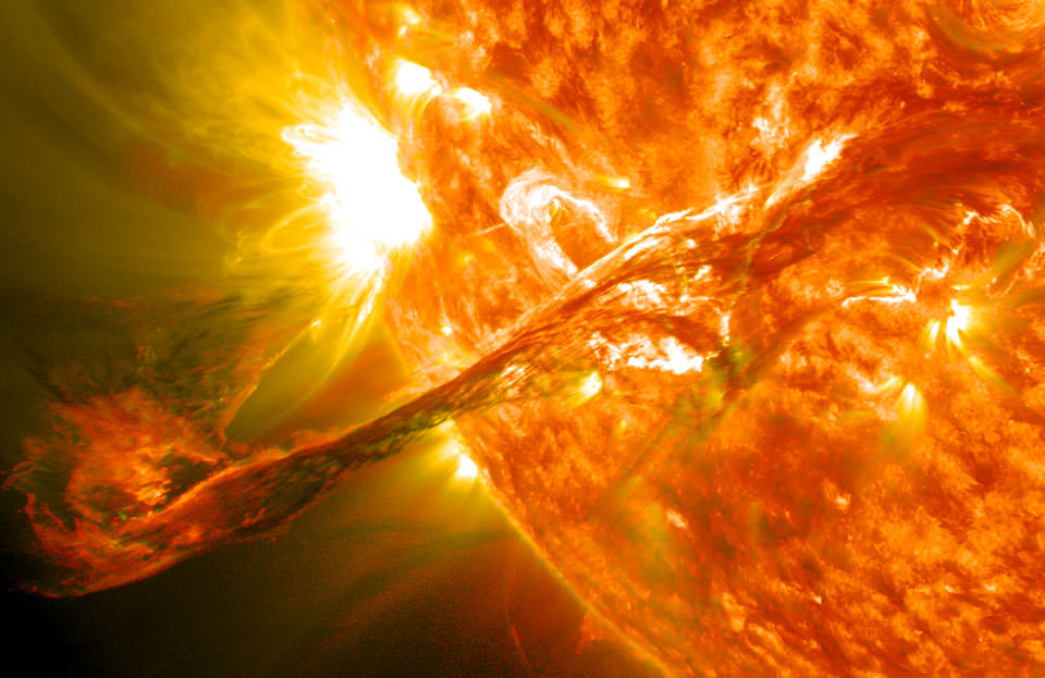
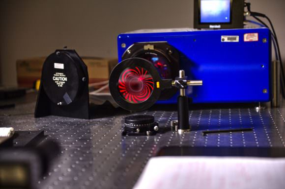
Scientists at NASA"s Goddard Space Flight Center are developing small, inexpensive optics to study the Sun's corona. Credit: NASA's GSFC, SDO AIA Team
Ever since astronomers first began using telescopes to get a better look at the heavens, they have struggled with a basic conundrum. In addition to magnification, telescopes also need to be able to resolve the small details of an object in order to help us get a better understanding of them. Doing this requires building larger and larger light-collecting mirrors, which requires instruments of greater size, cost and complexity.
However, scientists working at NASA Goddard’s Space Flight Center are working on an inexpensive alternative. Instead of relying on big and impractical large-aperture telescopes, they have proposed a device that could resolve tiny details while being a fraction of the size. It’s known as the photon sieve, and it is being specifically developed to study the Sun’s corona in the ultraviolet.
Basically, the photon sieve is a variation on the Fresnel zone plate, a form of optics that consist of tightly spaced sets of rings that alternate between the transparent and the opaque. Unlike telescopes which focus light through refraction or reflection, these plates cause light to diffract through transparent openings. On the other side, the light overlaps and is then focused onto a specific point – creating an image that can be recorded.
Image showing the photon sieve bringing red laser light to a pinpoint focus on its optical axis, and producing exotic diffraction patterns. Credits: NASA/W. Hrybyk
The photon sieve operates on the same basic principles, but with a slightly more sophisticated twist. Instead of thin openings (i.e. Fresnel zones), the sieve consists of a circular silicon lens that is dotted with millions of tiny holes. Although such a device would be potentially useful at all wavelengths, the Goddard team is specifically developing the photon sieve to answer a 50-year-old question about the Sun.
Essentially, they hope to study the Sun’s corona to see what mechanism is heating it. For some time, scientists have known that the corona and other layers of the Sun’s atmosphere (the chromosphere, the transition region, and the heliosphere) are significantly hotter than its surface. Why this is has remained a mystery. But perhaps, not for much longer.
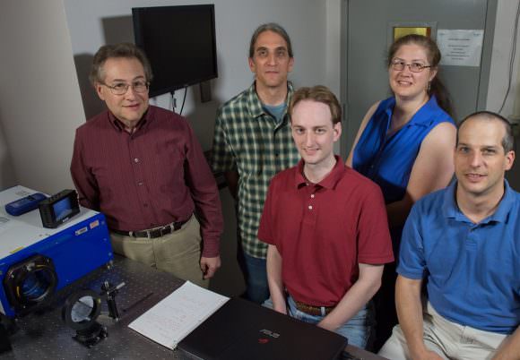
As Doug Rabin, the leader of the Goddard team, said in a NASA press release:
“This is already a success… For more than 50 years, the central unanswered question in solar coronal science has been to understand how energy transported from below is able to heat the corona. Current instruments have spatial resolutions about 100 times larger than the features that must be observed to understand this process.”
With support from Goddard’s Research and Development program, the team has already fabricated three sieves, all of which measure 7.62 cm (3 inches) in diameter. Each device contains a silicon wafer with 16 million holes, the sizes and locations of which were determined using a fabrication technique called photolithography – where light is used to transfer a geometric pattern from a photomask to a surface.
The Goddard team led by Doug Rabin (left) is working on a new optic device that will drastically reduce the size of telescopes. Credits: NASA/W. Hrybyk
However, in the long-run, they hope to create a sieve that will measure 1 meter (3 feet) in diameter. With an instrument of this size, they believe they will be able to achieve up to 100 times better angular resolution in the ultraviolet than NASA’s high-resolution space telescope – the Solar Dynamics Observatory. This would be just enough to start getting some answers from the Sun’s corona.
In the meantime, the team plans to begin testing to see if the sieve can operate in space, a process which should take less than a year. This will include whether or not it can survive the intense g-forces of a space launch, as well as the extreme environment of space. Other plans include marrying the technology to a series of CubeSats so a two-spacecraft formation-flying mission could be mounted to study the Sun’s corona.
In addition to shedding light on the mysteries of the Sun, a successful photon sieve could revolution optics as we know it. Rather than being forced to send massive and expensive apparatus’ into space (like the Hubble Space Telescope or the James Webb Telescope), astronomers could get all the high-resolution images they need from devices small enough to stick aboard a satellite measuring no more than a few square meters.
This would open up new venues for space research, allowing private companies and research institutions the ability to take detailed photos of distant stars, planets, and other celestial objects. It would also constitute another crucial step towards making space exploration affordable and accessible.
Earth's axial tilt (or obliquity) and its relation to the rotation axis and plane of orbit. Credit: Wikipedia Commons
In ancient times, the scholars, seers and magi of various cultures believed that the world took a number of forms – ranging from a ziggurat or a cube to the more popular flat disc surrounded by a sea. But thanks to the ongoing efforts of astronomers, we have come to understand that it is in fact a sphere, and one of many planets in a system that orbits the Sun.
Within the past few centuries, improvements in both scientific instruments and more comprehensive observations of the heavens have also helped astronomers to determine (with extreme accuracy) what the nature of Earth’s orbit is. In addition to knowing the precise distance from the Sun, we also know that our planet orbits the Sun with one pole constantly tilted towards it.
Earth’s Axis:
This is what is known axial tilt, where a planet’s vertical axis is tilted a certain degree towards the ecliptic of the object it orbits (in this case, the Sun). Such a tilt results in there being a difference in how much sunlight reaches a given point on the surface during the course of a year. In the case of Earth, the axis is tilted towards the ecliptic of the Sun at approximately 23.44° (or 23.439281° to be exact).
Earth’s axis points north to Polaris, the northern hemisphere’s North Star, and south to dim Sigma Octantis. Credit: Bob King
Seasonal Variations:
This tilt in Earth’s axis is what is responsible for seasonal changes during the course of the year. When the North Pole is pointed towards the Sun, the northern hemisphere experiences summer and the southern hemisphere experiences winter. When the South Pole is pointed towards the Sun, six months later, the situation is reversed.
In addition to variations in temperature, seasonal changes also result in changes to the diurnal cycle. Basically, in the summer, the day last longer and the Sun climbs higher in the sky. In winter, the days become shorter and the Sun is lower in the sky. In northern temperate latitudes, the Sun rises north of true east during the summer solstice, and sets north of true west, reversing in the winter. The Sun rises south of true east in the summer for the southern temperate zone, and sets south of true west.
The situation becomes extreme above the Arctic Circle, where there is no daylight at all for part of the year, and for up to six months at the North Pole itself (known as a “polar night”). In the southern hemisphere, the situation is reversed, with the South Pole oriented opposite the direction of the North Pole and experiencing what is known as a “midnight sun” (a day that lasts 24 hours).
The four seasons can be determined by the solstices (the point of maximum axial tilt toward or away from the Sun) and the equinoxes (when the direction of tilt and the Sun are perpendicular). In the northern hemisphere, winter solstice occurs around December 21st, summer solstice around June 21st, spring equinox around March 20th, and autumnal equinox on or about September 22nd or 23rd. In the southern hemisphere, the situation is reversed, with the summer and winter solstices exchanged and the spring and autumnal equinox dates swapped.
Changes Over Time:
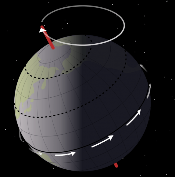
The angle of the Earth’s tilt is relatively stable over long periods of time. However, Earth’s axis does undergo a slight irregular motion known as nutation – a rocking, swaying, or nodding motion (like a gyroscope) – that has a period of 18.6 years. Earth’s axis is also subject to a slight wobble (like a spinning top), which is causing its orientation to change over time.
Known as precession, this process is causing the date of the seasons to slowly change over a 25,800 year cycle. Precession is not only the reason for the difference between a sidereal year and a tropical year, it is also the reason why the seasons will eventually flip. When this happens, summer will occur in the northern hemisphere during December and winter during June.
Artist’s rendition of the Earth’s rotation and the precession of the Equinoxes. Credit: NASA
Precession, along with other orbital factors, is also the reason for what is known as “length-of-day variation”. Essentially, this is a phenomna where the dates of Earth’s perihelion and aphelion (which currently take place on Jan. 3rd and July 4th, respectively) change over time. Both of these motions are caused by the varying attraction of the Sun and the Moon on the Earth’s equatorial region.
Needless to say, Earth’s rotation and orbit around the Sun are not as simple we once though. During the Scientific Revolution, it was a huge revelation to learn that the Earth was not a fixed point in the Universe, and that the “celestial spheres” were planets like Earth. But even then, astronomers like Copernicus and Galileo still believed that the Earth’s orbit was a perfect circle, and could not imagine that its rotation was subject to imperfections.
It’s only been with time that the true nature of our planet’s inclination and movements have come to be understood. And what we know is that they lead to some serious variations over time – both in the short run (i.e. seasonal change), and in the long-run.
The eccentricity in Mars' orbit means that it is . Credit: NASA
With the Scientific Revolution, astronomers became aware of the fact that the Earth and the other planets orbit the Sun. And thanks to Copernicus, Galileo, Kepler, and Newton, the study of their orbits was refined to the point of mathematical precision. And with the subsequent discoveries of Uranus, Neptune, Pluto and the Kuiper Belt Objects, we have come to understand just how varied the orbits of the Solar Planets are.
Consider Mars, Earth’s second-closest neighbor, and a planet that is often referred to as “Earth’s Twin”. While it has many things in common with Earth, one area in which they differ greatly is in terms of their orbits. In addition to being farther from the Sun, Mars also has a much more elliptical orbit, which results in some rather interesting variations in temperature and weather patterns.
Perihelion and Aphelion:
Mars orbits the Sun at an average distance (semi-major axis) of 228 million km (141.67 million mi), or 1.524 astronomical units (over one and a half times the distance between Earth and the Sun). However, Mars also has the second most eccentric orbit of all the planets in the Solar System (0.0934), which makes it a distant second to crazy Mercury (at 0.20563).
This means that Mars’ distance from the Sun varies between perihelion (its closest point) and aphelion (its farthest point). In short, the distance between Mars and the Sun ranges during the course of a Martian year from 206,700,000 km (128.437 million mi) at perihelion and 249,200,000 km (154.8457 million mi) at aphelion – or 1.38 AU and 1.666 AU.
Speaking of a Martian year, with an average orbital speed of 24 km/s, Mars takes the equivalent of 687 Earth days to complete a single orbit around the Sun. This means that a year on Mars is equivalent to 1.88 Earth years. Adjusted for Martian days (aka. sols) – which last 24 hours, 39 minutes, and 35 seconds – that works out to a year being 668.5991 sols long (still almost twice as long).
Mars in also the midst of a long-term increase in eccentricity. Roughly 19,000 years ago, it reached a minimum of 0.079, and will peak again at an eccentricity of 0.105 (with a perihelion distance of 1.3621 AU) in about 24,000 years. In addition, the orbit was nearly circular about 1.35 million years ago, and will be again one million years from now.
Axial Tilt:
Much like Earth, Mars also has a significantly tilted axis. In fact, with an inclination of 25.19° to its orbital plane, it is very close to Earth’s own tilt of 23.439°. This means that like Earth, Mars also experiences seasonal variations in terms of temperature. On average, the surface temperature of Mars is much colder than what we experience here on Earth, but the variation is largely the same.
Mars eccentric orbit and axial tilt result in considerable seasonal variations. Credit and Copyright: Encyclopedia Britannica
All told, the average surface temperature on Mars is -46 °C (-51 °F). This ranges from a low of -143 °C (-225.4 °F), which takes place during winter at the poles; and a high of 35 °C (95 °F), which occurs during summer and midday at the equator. This means that at certain times of the year, Mars is actually warmer than certain parts of Earth.
Orbit and Seasonal Changes:
Mars’ variations in temperature and its seasonal changes are also related to changes in the planet’s orbit. Essentially, Mars’ eccentric orbit means that it travels more slowly around the Sun when it is further from it, and more quickly when it is closer (as stated in Kepler’s Three Laws of Planetary Motion).
Mars’ aphelion coincides with Spring in its northern hemisphere, which makes it the longest season on the planet – lasting roughly 7 Earth months. Summer is second longest, lasting six months, while Fall and Winter last 5.3 and just over 4 months, respectively. In the south, the length of the seasons is only slightly different.
Mars is near perihelion when it is summer in the southern hemisphere and winter in the north, and near aphelion when it is winter in the southern hemisphere and summer in the north. As a result, the seasons in the southern hemisphere are more extreme and the seasons in the northern are milder. The summer temperatures in the south can be up to 30 K (30 °C; 54 °F) warmer than the equivalent summer temperatures in the north.
Mars’ south polar ice cap, seen in April 2000 by the Mars Odyssey probe. Credit: NASA/JPL/MSSS
It also snows on Mars. In 2008, NASA’s Phoenix Landerfound water ice in the polar regions of the planet. This was an expected finding, but scientists were not prepared to observe snow falling from clouds. The snow, combined with soil chemistry experiments, led scientists to believe that the landing site had a wetter and warmer climate in the past.
And then in 2012, data obtained by the Mars Reconnaissance Orbiter revealed that carbon-dioxide snowfalls occur in the southern polar region of Mars. For decades, scientists have known that carbon-dioxide ice is a permanent part of Mars’ seasonal cycle and exists in the southern polar caps. But this was the first time that such a phenomena was detected, and it remains the only known example of carbon-dioxide snow falling anywhere in our solar system.
For starters, soil samples and orbital observation have demonstrated conclusively that roughly 3.7 billion years ago, the planet had more water on its surface than is currently in the Atlantic Ocean. Similarly, atmospheric studies conducted on the surface and from space have proven that Mars also had a viable atmosphere at that time, one which was slowly stripped away by solar wind.
Scientists were able to gauge the rate of water loss on Mars by measuring the ratio of water and HDO from today and 4.3 billion years ago. Credit: Kevin Gill
Weather Patterns:
These seasonal variations allow Mars to experience some extremes in weather. Most notably, Mars has the largest dust storms in the Solar System. These can vary from a storm over a small area to gigantic storms (thousands of km in diameter) that cover the entire planet and obscure the surface from view. They tend to occur when Mars is closest to the Sun, and have been shown to increase the global temperature.
The first mission to notice this was the Mariner 9 orbiter, which was the first spacecraft to orbit Mars in 1971, it sent pictures back to Earth of a world consumed in haze. The entire planet was covered by a dust storm so massive that only Olympus Mons, the giant Martian volcano that measures 24 km high, could be seen above the clouds. This storm lasted for a full month, and delayed Mariner 9‘s attempts to photograph the planet in detail.
And then on June 9th, 2001, the Hubble Space Telescope spotted a dust storm in the Hellas Basin on Mars. By July, the storm had died down, but then grew again to become the largest storm in 25 years. So big was the storm that amateur astronomers using small telescopes were able to see it from Earth. And the cloud raised the temperature of the frigid Martian atmosphere by a stunning 30° Celsius.
These storms tend to occur when Mars is closest to the Sun, and are the result of temperatures rising and triggering changes in the air and soil. As the soil dries, it becomes more easily picked up by air currents, which are caused by pressure changes due to increased heat. The dust storms cause temperatures to rise even further, leading to Mars’ experiencing its own greenhouse effect.