In 2015, Russian billionaire Yuri Milner founded Breakthrough Initiatives with the intention of bolstering the search for extra-terrestrial life. Since that time, the non-profit organization – which is backed by Stephen Hawking and Mark Zuckerberg – has announced a number of advanced projects. The most ambitious of these is arguably Project Starshot, an interstellar mission that would make the journey to the nearest star in just 20 years.
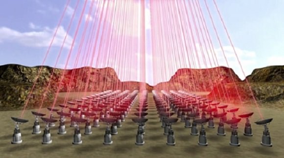
This concept involves an ultra-light nanocraft that would rely on a laser-driven sail to achieve speeds of up to 20% the speed of light. Naturally, for such a mission to be successful, a number of engineering challenges have to be tackled first. And according to a recent study by a team of international researchers, two of the most important issues are the shape of the sail itself, and the type of laser involved.
The researchers include Elena Popova of the Skobeltsyn Institute of Nuclear Physics in Moscow; Messoud Efendiev of the Institute of Computational Biology (ICB) at the German Research Center for Environmental Health (GmbH); and Ildar Gabitov of the Skoltech Center for Photonics and Quantum Materials in Moscow. Combining their expertise, they conducted a study that examined various stability models for this proposed mission.
As they indicate in their study, titled “On the Stability of a Space Vehicle Riding on an Intense Laser Beam“, the team ran stability simulations 0n the concept, taking into account the nature of the wafer-sized craft (aka. StarChip), the sail (aka. Lightsail) and the nature of the laser itself. For the sake of these simulations, they also factored in a number of assumptions about Starshot’s design.
These included the notion that the StarChip would be a rigid body (i.e. made up of solid material), that the circular sail would either be flat, spherical or conical (i.e. concave in shape), and that the surface of the sail would reflect the laser light. Beyond this, they played with multiple variations on the design, and came up with some rather telling results.
As Dr. Elena Popova, the lead author on the paper, told Universe Today via email:
“We considered different shapes of sail: a) spherical (coincides with parabolic for small sizes) as most appropriate for final configuration of nanocraft en route; b) conical; c) flat (simplest) (will be seen to be unstable so that even spinning of craft does not help).”
What they found was that the simplest, stable configuration would involve a sail that was spherical in shape. It would also require that the StarChip be tethered at a sufficient distance from the sail, one which would be longer than the curvature radius of the sail itself.
“For the sail with almost flat cone shape we obtained similar stability condition,” said Popova. “The nanocraft with flat sail is unstable in every case. It simply corresponds to the case of infinite radius of curvature of the sale. Hence, there is no way to extend center of mass beyond it.”
As for the laser, they considered several how the two main types would effect stability. This included uniform lasers that have a sharp boundary and “Gaussian” beams, which are characterized by high-intensity in the middle that declines rapidly towards the edges. As Dr. Popova stated, they determined that in order to ensure stability – and that the craft wouldn’t be lost to space – a uniform laser was the way to go.
“The nanocraft driven by intense laser beam pressure acting on its Lightsail is sensitive to the torques and lateral forces reacting on the surface of the sail. These forces influence the orientation and lateral displacement of the spacecraft, thus affecting its dynamics. If unstable the nanocraft might even be expelled from the area of laser beam. The most dangerous perturbations in the position of nanocraft inside the beam and its orientation relative to the beam axis are those with direct coupling between rotation and displacement (“spin-orbit coupling”).”
In the end, these were very similar to the conclusions reached by Professor Abraham Loeb and his colleagues at Starshot. In addition to being the Frank B. Baird, Jr. Professor of Science at Harvard University, Prof. Loeb is also the chairman of the Breakthrough Foundation’s Advisory Board. In a study titled “Stability of a Light Sail Riding on a Laser Beam” (published on Sept, 29th, 2016), they too examined what was necessary to ensure a stable mission.
This included the benefits of a conical vs. a spherical sail, and a uniform vs. a Gaussian beam. As Prof. Loeb told Universe Today via email:
“We found that a parachute-shaped sail riding on a Gaussian laser beam is unstable… We show in our paper that a sail shaped as a spherical shell (like a large ping-pong ball) can ride in a stable fashion on a laser beam that is shaped like a cylinder (or 3-4 lasers that establish a nearly circular illumination).”
As for the recommendations about the StarChip being at a sufficient distance from the LightSail, Prof. Loeb and his colleagues are of a different mind. “They argue that in case you attach a weight to the sail that is sufficiently well separated from the parachute, you might make it stable.” he said. “Even if this is true, it is unclear that their proposal is useful because such a configuration is rather complicated to build and launch.”
These are just a few of the engineering challenges facing an interstellar mission. Back in September, another study was released that assessed the risk of collisions and how it might effect the Starshot mission. In this case, the researchers suggested that the sail have a layer of shielding to absorb impacts, and that the laser array be used to clear debris in the LightSail’s path.
These conclusions echoed a similar study produced by Professor Phillip Lubin and his colleagues. A professor at the University of California, Santa Barbara (UCSB), Lubin is also one of the chief architects of Project Starshot and the mind behind the NASA-funded Directed Energy Propulsion for Interstellar Exploraiton (DEEP-IN) project and the Directed Energy Interstellar Study.
When Milner and the science team behind Starshot first announced their intention to create an interstellar spacecraft (in April 2016), they were met with a great deal of enthusiasm and skepticism. Understandably, many believed that such a mission was too ambitious, due to the challenges involved. But with every challenge that has been addressed, both by the Starshot team and outside researchers, the mission architecture has evolved.
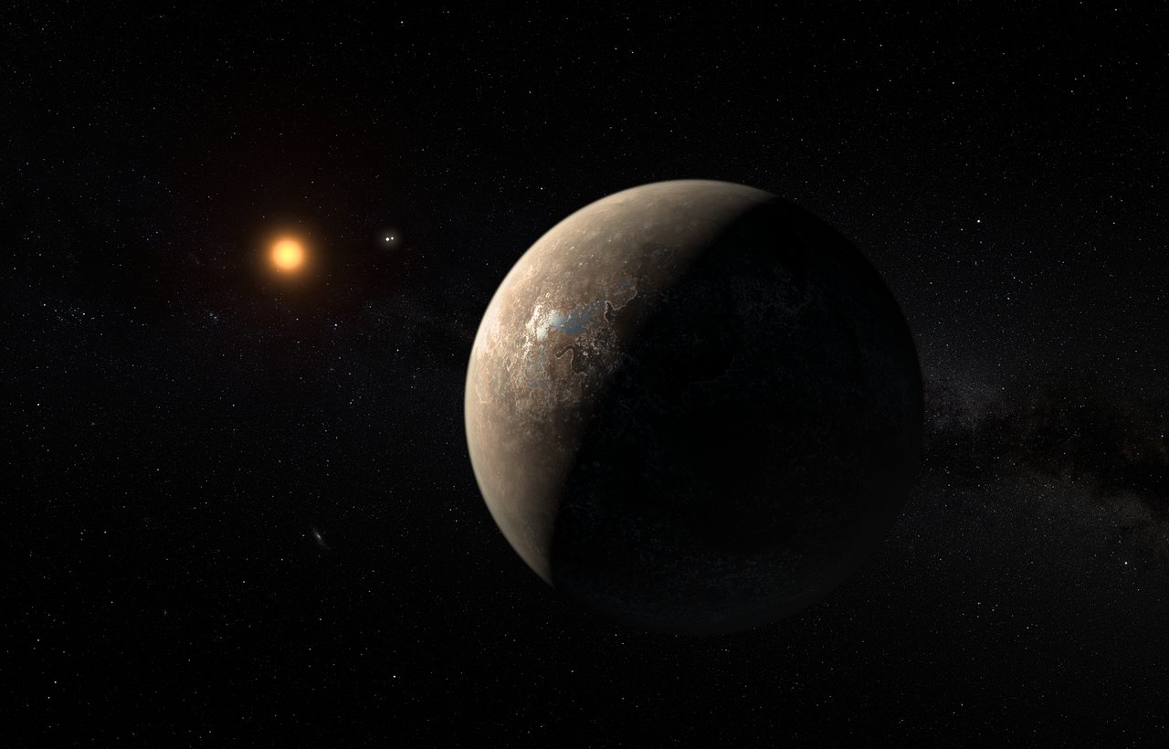
At this rate, barring any serious complications, we may be seeing an interstellar mission taking place within a decade or so. And, barring any hiccups in the mission, we could be exploring Alpha Centauri or Proxima b up close within our lifetime!
Further Reading: arXiv


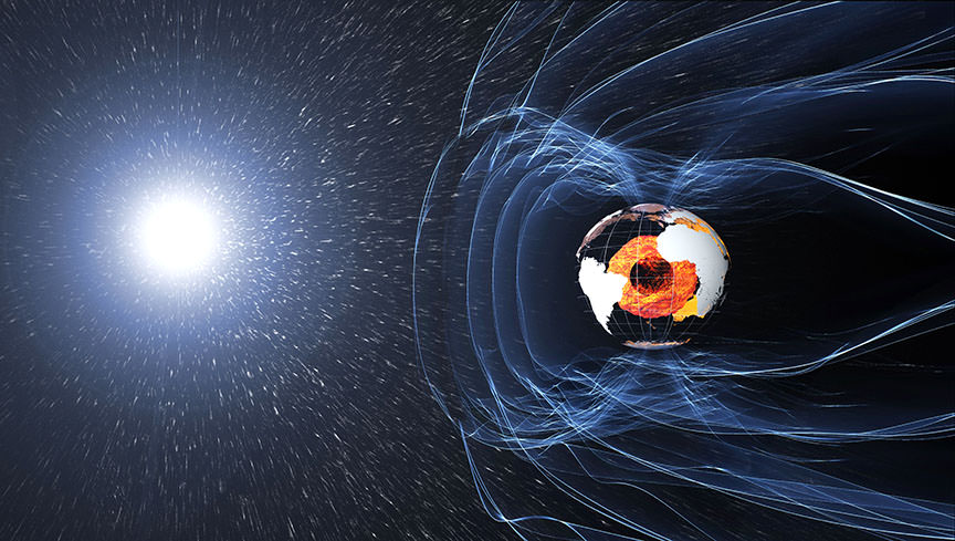
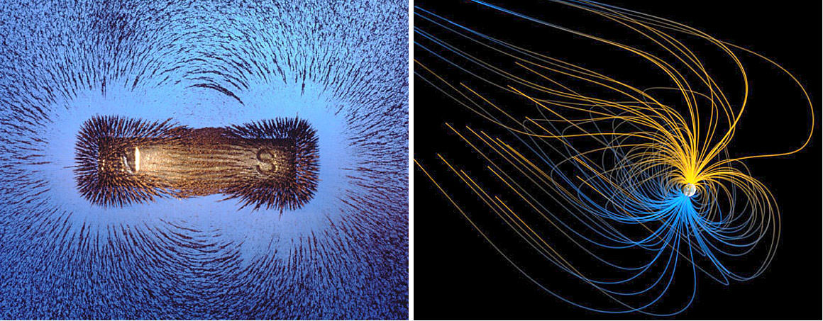

![Computer simulation of the Earth's field in a period of normal polarity between reversals.[1] The lines represent magnetic field lines, blue when the field points towards the center and yellow when away. The rotation axis of the Earth is centered and vertical. The dense clusters of lines are within the Earth's core](https://www.universetoday.com/wp-content/uploads/2010/03/Geodynamo_Between_Reversals-e1449100829326.gif)