Lake Asymmetry on Titan Explained

This mosaic of Cassini, SAR, ISS, and VIS images data shows that there are many more lakes in the northern regions of Titan than in the south. The eccentric orbit of Saturn is thought to have caused this imbalance. Image Credit: NASA/JPL/Caltech/University of Arizona/Cassini Imaging Team

If you’ve wanted to take a swim in a lake on Titan, don’t: they’re not lakes like we have here on Earth, composed of methane and ethane instead of water. If you have somehow evolved lungs to breathe and swim in these chemicals, you should take your beach vacation in the northern hemisphere of Titan, where you’ll find many more lakes. Data taken by the Cassini mission has shown that there are more of these methane lakes concentrated in the northern hemisphere of Saturn’s moon than in the southern hemisphere. A recent analysis of the Cassini findings by a team at Caltech has shown that the cause of this asymmetry of lakes is due to the orbit of Saturn.

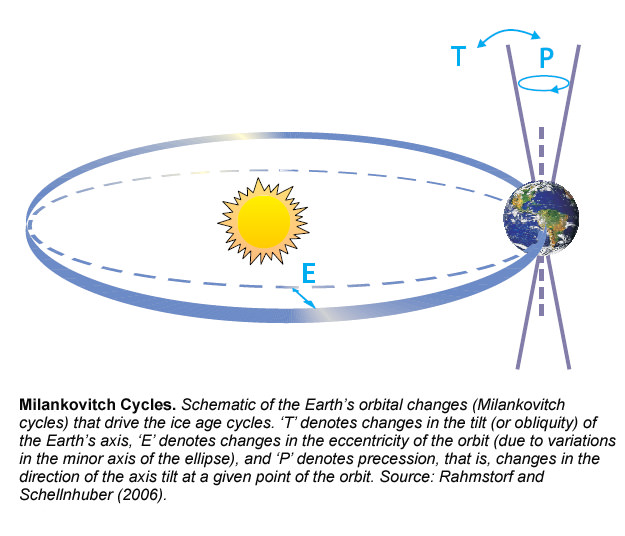
Because of the eccentricity of Saturn’s orbit around the Sun, there is a constant transfer of methane in Titan’s atmosphere from the south to the north. This effect is called astronomical climate forcing, or the Milankovitch cycle, and is thought to be the cause of ice ages here on Earth. We wrote about the Milankovitch cycles and their influence on climate change just earlier today.

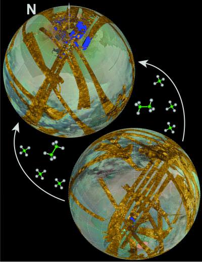
Scientists originally thought that the northern hemisphere was somehow differently structured than the south. Imaging data from Cassini showed that ethane and methane lakes cover 20 times more area in the northern hemisphere than lakes in the south. There also are more half-filled and dried-up lake beds in the north. For example, if the composition of the surface of Titan somehow allowed for more methane and ethane to permeate the ground more in the north, this could have explained the difference. But further data from Cassini has confirmed that there is no great difference in topography between the two hemispheres of Titan.

The seasonal differences on Titan only partially explain the asymmetry of lake formation. One year on Titan is 29.5 Earth years, so about every 15 years the seasons of Titan reverse. In other words, the winter and summer seasons could have caused the evaporation and transfer of gas to the north, where it is cooled and is currently in the form of lakes until the seasons change again.

A team led by Oded Aharonson, associate professor of planetary science at Caltech found that there was much more to the story, though. The seasonal effect could only account for changes in lake depth for each hemisphere to vary by about one meter. Titan’s lakes are hundreds of meters deep on average, and this process is too slow to explain the depth changes we see today. It became apparent that the seasonal differences were only partly contributing to this difference.

“On Titan, there are long-term climate cycles in the global movement of methane that make lakes and carve lake basins. In both cases we find a record of the process embedded in the geology,” Aharonson said in a press release.

The Milankovitch cycle on Titan is likely the cause of the lake imbalance. Summers in the north are long and relatively mild, while those in the south are shorter, but warmer. Over thousands of years, this leads to a net movement of gas towards the north, which then condenses and stays there in liquid form. During southern summer Titan is close to the sun, and during northern summer it is approximately 12% further from the Sun.

Their results appear in the advance online version of Nature Geoscience for November 29th. Animations detailing the transfer are available on Oded Aharonson’s home page.

If Cassini would have been sent to Titan 32,000 years ago, the picture would have been reversed: the south pole would have many more lakes than the north. Conversely, any Titanian deep-lake divers in a few thousand years will fare much better in the lakes of the south.

Source: Eurekalert, Oded Aharonson’s Home Page

Slow-Motion Supernova

This artist’s impression of a supernova shows the layers of gas ejected prior to the final deathly explosion of a massive star. Credit: NASA/Swift/Skyworks Digital/Dana Berry

[/caption]

Supernovae are generally considered as fast and furious events. For the Type II, core collapse supernovae, the core implodes almost instantaneously although it takes some time for the shockwave to escape the star. As it does, the star brightens in what’s known as the “rise time” of the supernova. For most Type II supernovae, this takes about a week.

So what are astronomers to make of supernova 2008iy that had an unprecedented rise time of at least 400 days?

From the time it was discovered, SN 2008iy was an oddball. When its spectra was analyzed, it was placed in the rare IIn subclass. This subclass is reserved for supernovae that feature narrow emission lines. Most supernovae have broad emission lines, if they even have emission lines at all.

To learn more about the history of this unusual case, astronomers at the University of California, Berkeley turned to archival images from the Palomar Quest survey. They searched images of the region to trace back the supernova as far as July of 2007, before which, the star was too faint to appear in images. Thus, the supernova brightening started at least that early and continued until late October of 2008 giving it a rise time at least four times as long as any previously discovered supernova.

The main clue to explain this mystery stemmed from the unusual emission lines. Generally, stars and supernovae are characterized by their absorption spectra which are caused when relatively cool gas stands between a hotter source and our detection. To generate emission lines, there must been a relatively dense medium being excited by the supernova. Furthermore, the fact that the lines were narrow implied that it was fairly motionless.

Together, this pointed to the progenitor undergoing a heightened period of mass loss prior to the detonation. The idea is such that the progenitor had shed large amounts of material. When the supernova occurred, this shell initially obscured the event. But as the ejecta from the supernova overtook the relatively stationary earlier shells, the brighter material slowly seeped out giving rise to the 400 day rise time.

While all stars undergo a period of mass loss in their post main sequence life, such a dense shell would be uncommon. To explain this, the authors turned to a type of star known as a Luminous Blue Variable. These stars are typically near the theoretical limit for the mass of a star (150 times the mass of the sun). Due to their extreme mass, they have strong stellar winds which periodically blow off large amounts of material that could create shells similar to those necessary for SN 2008iy. Unfortunately, this event was so distant that it could not be resolved to search for such a nebula. Even the host galaxy proved difficult to distinguish due to its faintness, although it is believed to be an irregular dwarf galaxy. Eta Carinae is one such luminous blue variable star. If perhaps one day soon it decides to turn into a supernova, it too will unfold in slow-motion.

What Color is Venus?

Venus. Image Credit: NASA/courtesy of nasaimages.org


Here’s a question: what color is Venus? With the unaided eye, Venus just looks like a very bright star in the sky. But spacecraft have sent back images of the cloud tops of Venus, and some have even returned images from the surface of Venus.

If you could actually fly out to Venus and look at it with your own eyes, you wouldn’t see much more than a bright white-yellowish ball with no features. You wouldn’t actually be able to see any of the cloud features that you can see in photographs of Venus. That’s because those photos are taken using different wavelengths of light, where differences in the cloud layers are visible. For example, the photo that accompanies this story was captured in the ultraviolet spectrum.

Although the atmosphere of Venus is almost entirely made up of carbon dioxide, the clouds that obscure our view to the surface are made of sulfur dioxide. These are opaque to visible light, and so we can’t see through them to the surface of Venus. These clouds actually rain droplets of sulfuric acid.

Surface of Venus by Venera.

If you could get down beneath the cloud tops of Venus, you wouldn’t be able to see much either. That’s because the clouds are so thick that most of the light from the Sun is blocked before it reaches the surface. You would see a dim landscape, like you might see at twilight. The surface of the planet is littered with brownish-red volcanic rocks. The bright red color you see in the Soviet Venera images of Venus have been brightened to show more surface detail.

So, what color is Venus? Yellowish-white.

We’ve written several articles about the color of the planets for Universe Today. Here’s an article about the color of Mercury, and here’s an article about the color of Pluto.

If you’d like more info on Venus, check out Hubblesite’s News Releases about Venus, and here’s a link to NASA’s Solar System Exploration Guide on Venus.

We’ve also recorded an entire episode of Astronomy Cast all about Venus. Listen here, Episode 50: Venus.

Amateur Spectroscopy

Credit: Robert Kaufman's image of Tarantula and Orion spectra (used with permission)

[/caption]

Amateur astronomers are a unique species worthy of their own reality TV show. Their craftsmanship, resourcefulness, dedication, and passion is simply amazing. Many professional astronomers rely heavily on amateurs for quick spot checks, discovery followups, collaboration on research projects, the diverse locations of their telescopes and their ability/willingness to put in long hours of observation. So what is spectroscopy, and what do the amateur astronomers get up to?

Absorption spectroscopy is the study of the color and light spectrum of stars and galaxies. We all love our Hubble photos and pretty astro-photographs, however most of the real research and science comes from observing the light spectrum.

Robin Leadbeater’s LHIRESIII Spectrograph

Robin Leadbeater's telescope with LHRESIII spectrograph

Astronomers look at emission lines and absorption lines in the spectra to determine the make up of stars, nebulas and galaxies. Dopler effects, orbital behavior, elements of stars, even atmospheres can be determined by observing these absorption and emission lines. Scientists believe that a carbon dioxide absorption spectrum line signature in the spectrum of a star with a transiting exo-planet could eventually be the most exciting discovery – a possible indicator of extra-terrestrial life.

Why are amateurs interested?

I asked Ken Harrison the moderator of the Yahoo group – Astronomical Spectroscopy, why amateurs would be interested in absorption spectra?

“I see it as the “last frontier” for amateur astronomers. When you’ve taken the 100th image of the Orion nebulae – what do you do next?? It’s challenging, interesting and can give some scientific value to your work. Amateurs have successfully recorded the spectra of nova before the professionals and complimented other variable star work with observations of the changing spectral emissions of stars showing their Doppler shifts and atmospheric changes.”

Ken specializes in the spectra of Wolf-Rayet stars and is currently writing a book on amateur spectroscopy. Ken has been building his own spectrographs since 1992 and has used a variety of devices ranging from a simple star analyzer on a digital SLR camera to a sophisticated guided spectrograph.

A spectrograph allows light to pass through a narrow slit where it is then split into it’s spectra by passing through some sort of diffraction grating, before being captured on a CCD. The plate scale of the CCD then comes into play as angstroms per pixel instead of the usual (astrometric measure) arc/secs per pixel.

Rob Kaufman recently captured a Nova outburst Nova Scuti 2009 (V496 SCT) between the trees and clouds from his back yard.

Rob Kaufman spectrograph of Nova Scuti 2009 (V496 SCT) outburst
Credit: Rob Kaufman's spectrogram of Nova Scuti 2009 (V496 SCT) outburst

Italian amateur Fulvio Mete has achieved a spectrographic separation of tight binary Beta Aurigea. The double Ha absorption line is easily identifiable in his image taken with a 14inch Celestron. Some of the world’s best telescopes are unable to separate Beta Aurigea optically, so being able to do a spectrographic separation with a back yard telescope is a significant achievement.

Fulvio Metes spectrograph of Beta Aurigae
Fulvio Mete's spectrogram of Beta Aurigae

Perhaps there is no finer example of the quality of the spectroscopy done by amateurs than the current citizen science project on the eclipse of binary Epsilon Aurigae. Robin Leadbeater from Three Hills Observatory, a team member/contributor to the Citizen Sky project and avid amateur astronomer, has documented the changing spectra of Epsilon Aurigae, in particular monitoring the changing KI (neutral potassium) 7699 absorption line during the early stages of the ingress.

Robin Leadbeater's Spectrogram of KI 7699 absorption line in Epsilon Aurigae eclipse.

The eclipse happens every 27 years and this eclipse will be the first to be fully documented with advanced spectroscopy – clearly alot of that will be performed by skillful amateurs.

So what equipment do I need?

Ken Harrison comments that the equipment required is not necessarily expensive and it is a lot of fun.

“Luckily with the filter gratings available at reasonable prices (Star Analyser, Rainbow Optics etc) interested amateurs can start using their current equipment with minimal cost and outlay. Freeware programs like IRIS (C Buil) and VSpec (V Desnoux) allow the detailed analysis of spectra to be done without all the mathematics or detailed physics. As experience grows so do the questions. What do those absorption features mean? Why does this spectrum look completely different from that spectrum? How can I get benn resolution? Yes, it has its learning curve like any new adventure, but there are many others who have trodden the road before and only too willing to assist  – To boldly go where few amateurs have gone before – Spectroscopy!!!”

Dale Mais another dedicated amateur from Orange Grove, San Diego County has an excellent paper on qualitative and quantitative analysis that can be achieved by amateur astronomers.

The contribution of amateurs across all forms of astronomy is significant, and spectroscopy is no exception. If you want more information join one of the Yahoo groups or major amateur astronomy forums as they all have discussion groups with experienced people who are keen to help you get started.

Special thanks to Ken Harrison, Robin Leadbeater, Rob Kaufman, Fulvio Mete and Dale Mais for your photos and insight!

Carnival of Space #131

This week’s Carnival of Space is hosted by John Williams over at Starry Critters

Click here to read the Carnival of Space #131.

And if you’re interested in looking back, here’s an archive to all the past Carnivals of Space. If you’ve got a space-related blog, you should really join the carnival. Just email an entry to [email protected], and the next host will link to it. It will help get awareness out there about your writing, help you meet others in the space community – and community is what blogging is all about. And if you really want to help out, let Fraser know if you can be a host, and he’ll schedule you into the calendar.

Finally, if you run a space-related blog, please post a link to the Carnival of Space. Help us get the word out.

An Astronomical Perspective on Climate Change

Ice cores and deep sea bed cores provide the best available record of changes in global temperature and CO2 content of the atmosphere going back 800,000 years. The data shows a clear periodicity in global temperatures which is thought to be linked to the Milankovitch cycle.

Back in 1920, Milutin Milankovitch, a Serbian mathematician, proposed that fine changes in Earth’s orbit around the Sun could explain an approximately 100,000 year cycle in glaciation seen from geological evidence. The tilt of the Earth’s axis swings slightly over a 41,000 year cycle – the eccentricity of Earth’s orbit moves from almost circular to more elliptical and back again over a 413,000 year cycle – and overlaying that you have not only the precession of the equinoxes, which is an inherent wobble in the Earth’s axial spin over a 26,000 year cycle, but also a precession of the whole of Earth’s orbit over a 23,000 year cycle.

Ice core data does show a rough concordance between glaciation and the synchronicity of these orbital cycles. Even though there’s no significant change in the mean amount of solar radiation reaching the Earth over the period of its annual orbit – the orbital changes can lead to increased polar shadowing and cooling.

Once ice does start advancing from the poles, a positive feedback loop can develop – since more ice increases the albedo of Earth’s surface and reflects more of the Sun’s heat back into space, thus reducing mean global temperatures.

ice coreIt’s thought that what limits the ice advancing is increasing CO2 in the atmosphere – which can be measured from trapped bubbles of air in the ice cores. More ice formation leads to less exposed land area for photosynthesis and silicate rock weathering to remove CO2 from the atmosphere. So the more ice that’s formed, the more CO2 accumulates in the atmosphere – which causes mean global temperatures to rise, which limits ongoing ice formation.

Of course the opposite is true in an ice-melting phase. Ice melting also follows a positive feedback loop since less ice means less albedo, meaning less solar radiation is reflected back into space and mean global temperatures rise. But again, CO2 becomes the limiting factor. With more exposed land, more CO2 is drawn from the atmosphere by photosynthesizing forests and rock weathering. A consequent drop in atmospheric CO2 cools the planet and hence limits ongoing ice melting.

But there lies the rub. We are in an ice-melting phase of the Milankovitch cycle now, where the Earth’s orbit is closer to circular and the Earth’s tilt is closer to perpendicular. But CO2 levels aren’t declining – partly because we’ve chopped a lot of trees and forests down, but mostly because of anthropogenic CO2 production. Without the limiting factor of declining CO2 we’ve seen in previous Milankovitch cycles, presumably the ice is just going to keep on melting as the albedo of the Earth surface declines.

Projected changes in coastlines with 170 metre sea level riseSo you might want to rethink that next coastal real estate purchase – or hope for the best from Copenhagen.

dotAstronomy Conference

I’m attending the .Astronomy (dotAstronomy) Conference this week Leiden, The Netherlands, where we are discussing novel concepts of thinking and working in astronomy today. We’ll be discussing the data deluge that will be produced by upcoming surveys and instruments, how citizen science is making a real impact, and the new ways of communicating science to the public with web 2.0, blogs, podcasts and social networking. All week, you can watch the morning sessions of .Astronomy online at UStream, (or watch the stream below) and check out the .Astronomy website here to see what talks you are interested in. You can ask questions via the UStream chat, or follow along with the .Astronomy Twitter feed. I’ll be giving a talk on the 365 Days of Astronomy on Friday morning.

Live video by Ustream

Solo Sailor Spots Pacific Bolide

Jessica Watson and Ellas Pink Lady
Jessica Watson and Ella's Pink Lady

A 16-year-old high school girl who is attempting to sail solo around the world spotted a bright bolide over the Pacific Ocean during the peak of last week’s Leonid meteor shower. The International Meteor organization relies on reports just like this from observers in the field….or in this case “all at sea”.

Jessica Watson a student from Queensland, Australia, has set off on the adventure of a lifetime, attempting to become the youngest woman to sail solo and unassisted around the world.

Continue reading “Solo Sailor Spots Pacific Bolide”

When Was Pluto Discovered?

Clyde Tombaugh

[/caption]
Five of the planets are visible with the unaided eye and have been known about for thousands of years. Uranus was discovered in 1781, and Neptune was found in 1846. but when was Pluto discovered?

Pluto was discovered February 18th, 1930 by Clyde Tombaugh at the Lowell Observatory in Flagstaff, Arizona. Now that Uranus and Neptune had been discovered, astronomers were certain that there were more planets in the outer Solar System. The director of the Lowell Observatory, Vesto Melvin Slipher, handed the job of finding this next planet, dubbed “Planet X” to the 23-year old Tombaugh.

Tombaugh used a tool called a “blink comparator” to compare two photographs of the night sky. He worked methodically, comparing two photographic plates, looking for any object that jumped from one night to another night. And finally on February 18th, 1930, Tombaugh discovered Pluto; a faint object in the right orbit.

The name for Pluto was chosen by an 11-year old British school girl named Venetia Burney. This continued the tradition of naming planets after Roman gods. Pluto was the Roman god of the underworld, the same as Hades in Greek mythology. It also matched the first initials of Percival Lowell, who the observatory was named after. Lowell died in 1916, and so he never saw the discovery of Pluto.

We have written many articles about the discovery of planets in the Solar System for Universe Today. Here’s an article about when Uranus was discovered, and here’s an article about when Neptune was discovered.

If you’d like more info on Pluto, check out Hubblesite’s News Releases about Pluto, and here’s a link to NASA’s Solar System Exploration Guide to Pluto.

We’ve also recorded a couple of episodes of Astronomy Cast about Pluto. Here’s a good one, Episode 64: Pluto and the Icy Outer Solar System.

When Was Jupiter Discovered?

Jupiter's Red Spot

[/caption]
Were you wondering when was Jupiter discovered? Well, there’s no way to know. Jupiter is one of the 5 planets visible with the unaided eye. If you go outside and Jupiter is up in the sky, it’s probably the brightest object up there, brighter than any star; only Venus is brighter. So the ancient people have known about Jupiter for thousands of years, and there’s no way to know when the first person noticed the planet.

Perhaps a better question to ask is, when did we realize that Jupiter was a planet? In ancient times, astronomers used to think that the Earth was the center of the Universe. This was the geocentric model. The Sun, the Moon, the planets, and even the stars all orbited around the Earth in a series of crystal shells. But one thing that was hard to explain was the strange movements of the planets. They would move in one direction, then stop and go backwards in a retrograde motion. Astronomers created ever more elaborate models to explain these bizarre movements.

But then in the 1500s Nicolaus Copernicus developed his model of a Sun-centered, or heliospheric model of the Solar System. The Sun was center of the Solar System, and the planets, including Earth and Jupiter orbited around it. This nicely explained the strange movements of the planets in the sky. They were really following a circular path around the Sun, but the Earth was also traveling around the Sun, and this created different speeds based on our perspective.

The first person to actually view Jupiter in a telescope was Galileo. Even with his rudimentary telescope, he was able to see bands across the planet, and the 4 large Galilean moons that have been named after him. The moons clearly were orbiting Jupiter, which broke the theory that everything in the Universe was orbiting the Earth.

With bigger telescopes, astronomers were able to see more details in Jupiter’s cloud tops and discover more moons. But it wasn’t until the space age that scientists got to really study Jupiter close up. NASA’s Pioneer 10 was the first spacecraft to fly past Jupiter in 1973. It passed within 34,000 km of the cloud tops.

We’ve written several articles about when the planets of the Solar System were discovered. Here’s an article about the discovery of Uranus, and here’s an article about the discovery of Neptune.

If you’d like more information on Jupiter, check out Hubblesite’s News Releases about Jupiter, and here’s a link to NASA’s Solar System Exploration Guide to Jupiter.

We’ve also recorded an entire episode of Astronomy Cast just about Jupiter. Listen here, Episode 56: Jupiter.

Reference:
NASA