Category: Earth Observation

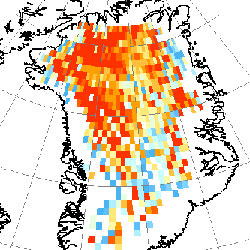
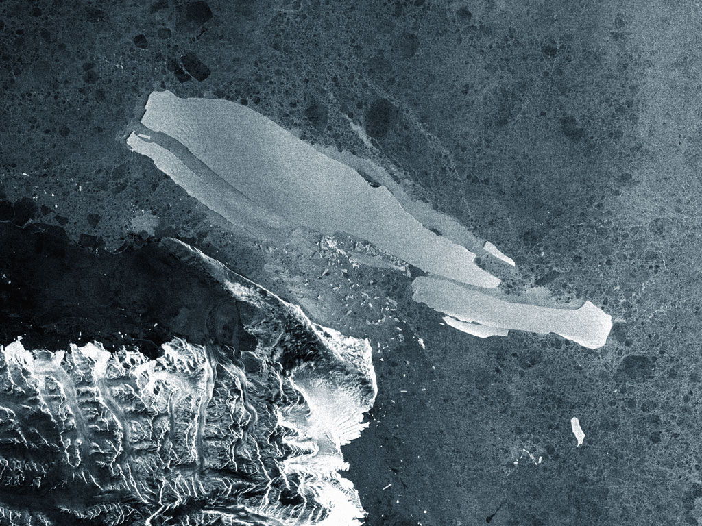
Decreasing levels of ice thickness from Greenland. Image credit: NASA/JPL. Click to enlarge.
In the first direct, comprehensive mass survey of the entire Greenland ice sheet, scientists using data from the NASA/German Aerospace Center Gravity Recovery and Climate Experiment (Grace) have measured a significant decrease in the mass of the Greenland ice cap. Grace is a satellite mission that measures movement in Earth’s mass.

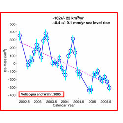
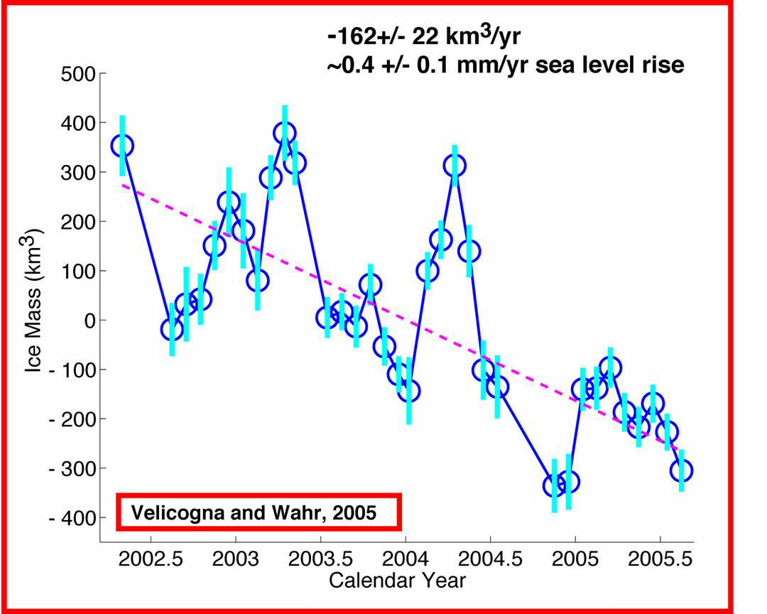
In an update to findings published in the journal Geophysical Research Letters, a team led by Dr. Isabella Velicogna of the University of Colorado, Boulder, found that Greenland’s ice sheet decreased by 162 (plus or minus 22) cubic kilometers a year between 2002 and 2005. This is higher than all previously published estimates, and it represents a change of about 0.4 millimeters (.016 inches) per year to global sea level rise.

“Greenland hosts the largest reservoir of freshwater in the northern hemisphere, and any substantial changes in the mass of its ice sheet will affect global sea level, ocean circulation and climate,” said Velicogna. “These results demonstrate Grace’s ability to measure monthly mass changes for an entire ice sheet ? a breakthrough in our ability to monitor such changes.”

Other recent Grace-related research includes measurements of seasonal changes in the Antarctic Circumpolar Current, Earth’s strongest ocean current system and a very significant force in global climate change. The Grace science team borrowed techniques from meteorologists who use atmospheric pressure to estimate winds. The team used Grace to estimate seasonal differences in ocean bottom pressure in order to estimate the intensity of the deep currents that move dense, cold water away from the Antarctic. This is the first study of seasonal variability along the full length of the Antarctic Circumpolar Current, which links the Atlantic, Pacific and Indian Oceans.

Dr. Victor Zlotnicki, an oceanographer at NASA’s Jet Propulsion Laboratory in Pasadena, Calif., called the technique a first step in global satellite monitoring of deep ocean circulation, which moves heat and salt between ocean basins. This exchange of heat and salt links sea ice, sea surface temperature and other polar ocean properties with weather and climate-related phenomena such as El Ninos. Some scientific studies indicate that deep ocean circulation plays a significant role in global climate change.

The identical twin Grace satellites track minute changes in Earth’s gravity field resulting from regional changes in Earth’s mass. Masses of ice, air, water and solid Earth can be moved by weather patterns, seasonal change, climate change and even tectonic events, such as this past December’s Sumatra earthquake. To track these changes, Grace measures micron-scale changes in the 220-kilometer (137-mile) separation between the two satellites, which fly in formation. To limit degradation of Grace’s satellite antennas due to atomic oxygen exposure and thereby preserve mission life, a series of maneuvers was performed earlier this month to swap the satellites’ relative positions in orbit.

In a demonstration of the satellites’ sensitivity to minute changes in Earth’s mass, the Grace science team reported that the satellites were able to measure the deformation of the Earth’s crust caused by the December 2004 Sumatra earthquake. That quake changed Earth’s gravity by one part in a billion.

Dr. Byron Tapley, Grace principal investigator at the University of Texas at Austin, said that the detection of the Sumatra earthquake gravity signal illustrates Grace’s ability to measure changes on and within Earth’s surface. “Grace’s measurements will add a global perspective to studies of large earthquakes and their impacts,” said Tapley.

Grace is managed for NASA by JPL. The University of Texas Center for Space Research has overall mission responsibility. GeoForschungsZentrum Potsdam, or GFZ, Potsdam, Germany, is responsible for German mission elements. Science data processing, distribution, archiving and product verification are managed jointly by JPL, the University of Texas and GFZ.

Imagery related to these latest Grace findings may be viewed at: http://www.nasa.gov/vision/earth/lookingatearth/grace-images-20051220.html .

For more information on Grace, visit: http://www.csr.utexas.edu/grace or http://www.gfz-potsdam.de/grace .

Original Source: NASA News Release

Earth’s northern lights. Image credit: Philippe Moussette.Click to enlarge
After some 400 years of relative stability, Earth’s North Magnetic Pole has moved nearly 1,100 kilometers out into the Arctic Ocean during the last century and at its present rate could move from northern Canada to Siberia within the next half-century.

If that happens, Alaska may be in danger of losing one of its most stunning natural phenomena – the Northern Lights.

But the surprisingly rapid movement of the magnetic pole doesn’t necessarily mean that our planet is going through a large-scale change that would result in the reversal of the Earth’s magnetic field, Oregon State University paleomagnetist Joseph Stoner reported at the annual meeting of the American Geophysical Union in San Francisco, Calif.

“This may be part of a normal oscillation and it will eventually migrate back toward Canada,” said Stoner, an assistant professor in OSU’s College of Oceanic and Atmospheric Sciences. “There is a lot of variability in its movement.”

Calculations of the North Magnetic Pole’s location from historical records goes back only about 400 years, while polar observations trace back to John Ross in 1838 at the west coast of Boothia Peninsula. To track its history beyond that, scientists have to dig into the Earth to look for clues.

Stoner and his colleagues have examined the sediment record from several Arctic lakes. These sediments – magnetic particles called magnetite – record the Earth’s magnetic field at the time they were deposited. Using carbon dating and other technologies – including layer counting – the scientists can determine approximately when the sediments were deposited and track changes in the magnetic field.

The Earth last went through a magnetic reversal some 780,000 years ago. These episodic reversals, in which south becomes north and vice versa, take thousands of years and are the result of complex changes in the Earth’s outer core. Liquid iron within the core generates the magnetic field that blankets the planet.

Because of that field, a compass reading of north in Oregon will be approximately 17 degrees east from “true geographic north.” In Florida, farther away and more in line with the poles, the declination is only 4-5 degrees west.

The Northern Lights, which are triggered by the sun and fixed in position by the magnetic field, drift with the movement of the North Magnetic Pole and may soon be visible in more southerly parts of Siberia and Europe – and less so in northern Canada and Alaska.

In their research, funded by the National Science Foundation, Stoner and his colleagues took core samples from several lakes, but focused on Sawtooth Lake and Murray Lake on Ellesmere Island in the Canadian Arctic. These lakes, about 40 to 80 meters deep, are covered by 2-3 meters of ice. The researchers drill through the ice, extend their corer down through the water, and retrieve sediment cores about five meters deep from the bottom of the lakes.

The 5-meter core samples provide sediments deposited up to about 5,000 years ago. Below that is bedrock, scoured clean by ice about 7,000 to 8,000 years ago.

“The conditions there give us nice age control,” Stoner said. “One of the problems with tracking the movement of the North Magnetic Pole has been tying the changes in the magnetic field to time. There just hasn’t been very good time constraint. But these sediments provide a reliable and reasonably tight timeline, having consistently been laid down at the rate of about one millimeter a year in annual layers.

“We’re trying to get the chronology down to a decadal scale or better.”

What their research has told Stoner and his colleagues is that the North Magnetic Pole has moved all over the place over the last few thousand years. In general, it moves back and forth between northern Canada and Siberia. But it also can veer sideways.

“There is a lot of variability in the polar motion,” Stoner pointed out, “but it isn’t something that occurs often. There appears to be a ‘jerk’ of the magnetic field that takes place every 500 years or so. The bottom line is that geomagnetic changes can be a lot more abrupt than we ever thought.”

Shifts in the North Magnetic Pole are of interest beyond the scientific community. Radiation influx is associated with the magnetic field, and charged particles streaming down through the atmosphere can affect airplane flights and telecommunications.

Original Source: NASA Astrobiology

The ozone hole: 2005. Image credit: NASA. Click to enlarge
NASA researchers, using data from the agency’s AURA satellite, determined the seasonal ozone hole that developed over Antarctica this year is smaller than in previous years.

NASA’s 2005 assessment of the size and thickness of the ozone layer was the first based on observations from the Ozone Monitoring Instrument on the agency’s Aura spacecraft. Aura was launched in 2004.

This year’s ozone hole measured 9.4 million square miles at its peak between September and mid-October, which was slightly larger than last year’s peak. The size of the ozone hole in 1998, the largest ever recorded, averaged 10.1 million square miles. For 10 of the past 12 years, the Antarctic ozone hole has been larger than 7.7 million square miles. Before 1985, it measured less than 4 million square miles.

The protective ozone layer over Antarctica annually undergoes a seasonal change, but since the first satellite measurements in 1979, the ozone hole has gotten larger. Human-produced chlorine and bromine chemicals can lead to the destruction of ozone in the stratosphere. By international agreement, these damaging chemicals were banned in 1995, and their levels in the atmosphere are decreasing.

Another important factor in how much ozone is destroyed each year is the temperature of the air high in the atmosphere. As with temperatures on the ground, some years are colder than others. When it’s colder in the stratosphere, more ozone is destroyed. The 2005 ozone hole was approximately 386,000 square miles larger than it would have been in a year with normal temperatures, because it was colder than average. Only twice in the last decade has the ozone hole shrunk to the size it typically was in the late 1980s. Those years, 2002 and 2004, were the warmest of the period.

Scientists also monitor how much ozone there is in the atmosphere from the ground to space. The thickness of the Antarctic ozone layer was the third highest of the last decade, as measured by the lowest reading recorded during the year. The level was 102 Dobson Units (the system of measurement designated to gauge ozone thickness). That is approximately one-half as thick as the layer before 1980 during the same time of year.

The Ozone Monitoring Instrument is the latest in a series of ozone-observing instruments flown by NASA over the last two decades. This instrument provides a more detailed view of ozone and is also able to monitor chemicals involved in ozone destruction. The instrument is a contribution to the mission from the Netherlands’ Agency for Aerospace Programs in collaboration with the Finnish Meteorological Institute. The Royal Netherlands Meteorological Institute is the principal investigator on the instrument.

For more information on NASA’s Aura mission on the Web, visit:
http://www.nasa.gov/aura

Original Source: NASA News Release

Artist’s impression of Earth auroras. Image credit: NASA Click to enlarge
Scientists from NASA and the National Science Foundation discovered a way to combine ground and space observations to create an unprecedented view of upper atmosphere disturbances during space storms.

Large, global-scale disturbances resemble weather cold fronts. They form in the Earth’s electrified upper atmosphere during space storms. The disturbances result from plumes of electrified plasma that form in the ionosphere. When the plasma plumes pass overhead, they impede low and high frequency radio communications and delay Global Positioning System navigation signals.

“Previously, they seemed like random events,” said John Foster, associate director of the Massachusetts Institute of Technology’s Haystack Observatory. He is principal investigator of the Foundation supported Millstone Hill Observatory, Wesford, Mass.

“People knew there was a space storm that must have disrupted their system, but they had no idea why,” said Tony Mannucci, group supervisor of Ionospheric and Atmospheric Remote Sensing at NASA’s Jet Propulsion Laboratory, Pasadena, Calif. “Now we know it’s not just chaos; there is cause and effect. We are beginning to put together the full picture, which will ultimately let us predict space storms.”

Predicting space weather is a primary goal of the National Space Weather Program involving NASA, the foundation and several other federal agencies. The view researchers created allowed them to link movement of the plumes to processes that release plasma into space. “Discovering this link is like discovering the movement of cold fronts is responsible for sudden thunderstorms,” said Jerry Goldstein, principal scientist at the Southwest Research Institute, San Antonio.

Since the occurrence of plasma plumes in the ionosphere disrupts GPS signals, they provide a continuous monitor of these disturbances. Researchers discovered a link between GPS data and satellite images of the plasmasphere. The plasmasphere is a plasma cloud surrounding Earth above the ionosphere. It is being observed from NASA’s Imager for Magnetopause to Aurora Global Exploration satellite. The researchers discovered the motion of the ionospheric plumes corresponded to the ejection of plasma from the plasmasphere during space storms.

The combined observations allowed construction of an underlying picture of the processes during space storms, when the Earth’s magnetic field is buffeted by hot plasma from the sun. As the solar plasma blows by, it generates an electric field that is transmitted to the plasmasphere and ionosphere. This electric field propels the ionospheric and the plasmaspheric plasma out into space. For the first time, scientists can directly connect the plasma observed in the ionosphere with the plasmasphere plumes that extend many thousand of kilometers into space.

“We also know these disturbances occur most often between noon and dusk, and between mid to high latitudes, due to the global structure of the electric and magnetic fields during space storms,” said Anthea Coster of the Haystack Observatory. “Ground and space based, and in situ measurements are allowing scientists to understand the ionosphere-thermosphere-magnetosphere as a coupled system.”

The plumes degrade GPS signals in two primary ways. First, they cause position error by time delaying the propagation of GPS signals. Second, the turbulence they generate causes receivers to lose the signal through an effect known as scintillation. It is similar to the apparent twinkling of stars caused by atmospheric turbulence.

Researchers are presenting the findings today during the American Geophysical Union meeting in San Francisco, Calif. For information about space weather and other research on the Web, visit:
http://www.nasa.gov/vision/universe/solarsystem/cold_front.html

Original Source: NASA News Release

Earth. Image credit: NASA Click to enlarge
The history of life on Earth is closely linked to the appearance of oxygen in the atmosphere. The current scientific consensus holds that significant amounts of oxygen first appeared in Earth’s atmosphere some 2.4 billion years ago, with a second large increase in atmospheric oxygen occurring much later, perhaps around 600 million years ago.

However, new findings by University of Maryland geologists suggest that the second jump in atmospheric oxygen actually may have begun much earlier and occurred more gradually than previously thought. The findings were made possible using a new tool for tracking microbial life in ancient environments developed at Maryland. Funded by the National Science Foundation and NASA, the work appears in the December 2 issue of Science.

Graduate researcher David Johnston, research scientist Boswell Wing and colleagues in the University of Maryland’s department of geology and Earth System Science Interdisciplinary Center led an international team of researchers that used high-precision measurements of a rare sulfur isotope, 33S, to establish that ancient marine microbes known as sulfur disproportionating prokaryotes were widely active almost 500 million years earlier than previously thought.

The intermediate sulfur compounds used by these sulfur disproportionating bacteria are formed by the exposure of sulfide minerals to oxygen gas. Thus, evidence of widespread activity by this type of bacteria has been interpreted by scientists as evidence of increased atmospheric oxygen content.

“These measurements imply that sulfur compound disproportionation was an active part of the sulfur cycle by [1.3 million years ago], and that progressive Earth surface oxygenation may have characterized the [middle Proterozoic],” the authors write.

The Proterozoic is the period in Earth’s history from about 2.4 billion years ago to 545 million years ago.

“The findings also demonstrate that the new 33S-based research method can be used to uniquely track the presence and character of microbial life in ancient environments and provide a glimpse of evolution in action,” said Johnston. “This approach provides a significant new tool in the astrobiological search for early life on Earth and beyond.”

The Air That We Breathe

When our planet formed some 4.5 billion years ago, virtually all the oxygen on Earth was chemically bound to other elements. It was in solid compounds like quartz and other silicate minerals, in liquid compounds like water, and in gaseous compounds like sulfur dioxide and carbon dioxide. Free oxygen — the gas that allows us to breath, and which is essential to all advanced life — was practically non-existent.

Scientists have long thought that appearance of oxygen in the atmosphere was marked by two distinct jumps in oxygen levels. In recent years, researchers have used a method developed by University of Maryland geologist James Farquhar and Maryland colleagues to conclusively determine that significant amounts of oxygen first appeared in Earth’s atmosphere some 2.4 billion years ago. Sometimes referred to as the “Great Oxidation Event,” this increase marks the beginning of the Proterozoic period.

A general scientific consensus has also held that the second major rise in atmospheric oxygen occurred some 600 million years ago, with oxygen rising to near modern levels at that time. Evidence of multicellular animals first appears in the geologic around this time.

“There has been a lot of discussion about whether the second major increase in atmospheric oxygen was quick and stepwise, or slow and progressive,” said Wing. “Our results support the idea that the second rise was progressive and began around 1.3 billion years ago, rather than 0.6 billion years ago.”

In addition to Johnston, Wing’s Maryland co-authors on the Dec. 2 paper are geology colleagues James Farquhar and Jay Kaufman. Their group works to document links between sulfur isotopes and the evolution of Earth’s atmosphere using a combination of field research, laboratory analysis of rock samples, geochemical models, photochemical experiments with sulfur-bearing gases and microbial experiments.

“Active microbial sulfur disproportionation in the Mesoproterozoic” by David T. Johnston, Boswell A. Wing, James Farquhar and Alan J. Kaufman, University of Maryland; Harald Strauss, Universit?t M?nster; Timothy W. Lyons, University of California, Riverside; Linda C. Kah, University of Tennessee; Donald E. Canfield, Southern Denmark University: Science, Dec. 2, 2005.

Original Source: UM News Release

Earth and Moon system as seen by VIRTIS-M. Image credit: ESA Click to enlarge
A recent check of the VIRTIS imaging spectrometer during the Venus Express commissioning phase has allowed its first remote-sensing data to be acquired, using Earth and the Moon as a reference.

After a successful in-flight checkout of the spacecraft’s systems in the first ten days of flight, the ESOC operations team is now verifying the health and functioning of all the Venus Express instruments. These observations were made as part of this checkout.

Of course the very large distance that Venus Express has travelled since its launch makes these images of limited interest to the general public, but to the scientific team it confirms the excellent operation of their instrument.

This gives them confidence of spectacular results when the spacecraft reaches Venus where similar measurements will be made hundreds times closer.

Only two weeks after the launch, VIRTIS, the Ultraviolet/Visible/Near-Infrared mapping spectrometer, has been able to make its first planetary observations, capturing the Earth-Moon system.

“The observations were made from 3.5 million kilometres away, with a phase angle of 65 degrees, meaning that 65% of the Earth’s disk was illuminated by the Sun, providing observations of both the day and night sides of the Earth,” explains Guiseppe Piccioni, one of the two Principal Investigators (PI).

These Earth observations will be used to test the instrument on a real planetary case, before Venus approach.

“A comparison of Venus spectra with Earth spectra with the same instrument will also be of interest for textbook illustration of the comparison between the two planets,” explained Pierre Drossart, the other PI.

The Moon has also been observed, providing additional observations of particular interest for calibrating the intrument.

The VIRTIS instrument on Venus Express is a twin of the same instrument on Rosetta, and similar observations were sent back by Rosetta in March 2005, so comparisons of the two sets of observations will be very useful for calibration purposes. The VIRTIS instrument is led jointly by INAF-IASF, Rome, Italy, and Observatoire de Paris, France.

Original Source: ESA Portal

The Earth. Image credit: NASA Click to enlarge
A surprising new study by an international team of researchers has concluded Earth’s continents most likely were in place soon after the planet was formed, overturning a long-held theory that the early planet was either moon-like or dominated by oceans.

The team came to the conclusion following an analysis of a rare metal element known as hafnium in ancient minerals from the Jack Hills in Western Australia, thought to be among the oldest rocks on Earth. Hafnium is found in association with zircon crystals in the Jack Hills rocks, which date to almost 4.4 billion years ago.

“These results support the view that the continental crust had formed by 4.4-4.5 billion years ago and was rapidly recycled into the mantle,” the researchers wrote in Science Express. Led by Professor Mark Harrison of the Australian National University, the team also included University of Colorado Assistant Professor Stephen Mojzsis and researchers from the University of California, Los Angeles and Ecole Normale Superieure University in France.

The researchers used hafnium as a “tracer” element, using isotopes to infer the existence of early continental formation on Earth dating to Hadeon Eon, which took place during the first 500 million years of Earth’s history, said Mojzsis, an assistant professor of geological sciences at CU-Boulder. Mojzsis also is a member of CU-Boulder’s Center for Astrobiology.

“The evidence indicates that there was substantial continental crust on Earth within its first 100 million years of existence,” said Mojzsis. “It looks like the Earth started off with a bang.”

A 2001 study led by Mojzsis published in the journal Nature showed evidence for the presence of water on Earth’s surface roughly 4.3 billion years ago. “The view we are taking now is that Earth’s crust, oceans and atmosphere were in place very early on, and that a habitable planet was established rapidly,” said Mojzsis.

The work was supported in part by a grant from NASA’s Exobiology Program.

Original Source: CU-Boulder News Release

The Earth. Image credit: NASA. Click to enlarge
New ANU research is set to radically overturn the conventional wisdom that early Earth was a hellish planet barren of continents.

An international research team led by Professor Mark Harrison of the Research School of Earth Sciences analysed unique 4 to 4.35 billion-year-old minerals from outback Australia and found evidence that a fringe theory detailing the development of continents during the first 500 million years of Earth history – the Hadean (“hellish”) Eon – is likely to be correct.

The research, published in the latest edition of Science, follows on from results by Professor Harrison and his colleagues published earlier this year that confirmed that our planet was also likely to have had oceans during most of the Hadean.

“A new picture of early Earth is emerging,” Professor Harrison said. “We have evidence that the Earth’s early surface supported water – the key ingredient in making our planet habitable. We have evidence that this water interacted with continent-forming magmas throughout the Hadean.

“And now we have evidence that massive amounts of continental crust were produced almost immediately upon Earth formation. The Hadean Earth may have looked much like it does today rather than our imagined view of a desiccated world devoid of continents.”

Professor Harrison and his team gathered their evidence from zircons, the oldest known minerals on Earth, called zircons. These ancient grains, typically about the width of a human hair, are found only in the Murchison region of Western Australia. The team analysed the isotopic properties of the element hafnium in about 100 tiny zircons that are as old as 4.35 billion years.

Conventionally, it has been believed that the Earth’s continents developed slowly over a long period of time beginning about 4 billion years ago – or 500 million years after the planet formed.

However, hafnium isotope variations produced by the radioactive decay of an isotope of lutetium indicate many of these ancient zircons formed in a continental setting within about 100 million years of Earth formation.

“The evidence points to almost immediate development of continent followed by its rapid recycling back into the mantle via a process akin to modern plate tectonics,” according to Professor Harrison.

The isotopic imprint left on the mantle by early melting shows up again in younger zircons – providing evidence that they have tapped the same source. This suggests that the amount of mantle processed to make continent must have been enormous.

“The results are consistent with the Earth hosting a similar mass of continental crust as the present day at 4.5-4.4 billion years.

“This is a radical departure from conventional wisdom regarding the Hadean Earth,” said Professor Harrison.

“But these ancient zircons represent the only geological record we have for that period of Earth history and thus the stories they tell take precedence over myths that arose in the absence of observational evidence.”

“The simplest explanation of all the evidence is that essentially from its formation, the planet fell into a dynamic regime that has persisted to the present day.”

Original Source: ANU News Release

B-15A Iceberg breaking up. Image credit: ESA. Click to enlarge.
After five years of being the world’s largest free-floating object, the B-15A iceberg has broken into smaller pieces off Antarctica’s Cape Adare.

ESA’s Envisat satellite’s Advanced Synthetic Aperture Radar (ASAR) is sensitive to ice, and has been tracking the movement of the drifting ice object continuously since the beginning of this year. Its latest imagery reveals the bottle-shaped iceberg split into nine knife-shaped icebergs and a myriad of smaller pieces on 27-28 October, the largest being formed by fractures along the long axis of the original single iceberg.

Measuring – until last week – around 115 kilometres in length with an area exceeding 2500 square kilometres, the B-15A tabular iceberg had apparently run aground off Cape Adare, the northernmost corner of the Victoria Land Coast. This stranding appears to have led to flexing and straining which resulted in the break-up.

“The long knife-shaped pieces suggest the iceberg has split along existing lines of weakness within the iceberg,” says Mark Drinkwater of ESA’s Ocean and Ice Unit. “These would have been pre-existing fractures and crevasses in the ice shelf.”

These new icebergs, named by the US National Oceanic and Atmospheric Administration (NOAA) National Ice Center, will retain their parent’s title: the three largest island-sized pieces have been called B-15M, B-15N and B-15P.

B-15A was the largest remaining section of the even larger B-15 iceberg that calved from the nearby Ross Ice Shelf in March 2000 before breaking up into smaller sections off McMurdo Island.

Since then its B-15A section drifted into McMurdo Sound, where its presence blocked ocean currents and led to a build-up of sea ice that decimated local penguin colonies, deprived of open waters for feeding. During the spring of this year prevailing currents took B-15A slowly past the Drygalski ice tongue. A full-fledged collision failed to take place, but a glancing blow broke the end off Drygalski in mid-April.

The iceberg sailed on to have a less-destructive close encounter with the Aviator Glacier ice tongue at Lady Newnes Bay before becoming stranded off Cape Adare in mid-October.

Radar monitoring of Antarctic ice
ASAR is extremely useful for tracking changes in polar ice. ASAR can peer through the thickest polar clouds and work through local day and night. And because it measures surface texture, the instrument is also extremely sensitive to different types of ice – so the radar image clearly delineates the older, rougher surface of icebergs from surrounding sea ice, while optical sensors simply show a continuity of snow-covered ice.

Envisat’s ASAR instrument monitors Antarctica in two different modes: Global Monitoring Mode (GMM) provides 400-kilometre swath one-kilometre resolution images, enabling rapid mosaicking of the whole of Antarctica to monitor changes in sea ice extent, ice shelves and iceberg movement.

Wide Swath Mode (WSM) possesses the same swath but with 150-metre resolution for a detailed view of areas of particular interest.

ASAR GMM images are routinely provided to a variety of users including the National Ice Center, responsible for tracking icebergs worldwide.

Original Source: ESA News Release

Map of Greenland with temperature changes. Image credit: ESA. Click to enlarge.
Researchers have utilised more than a decade’s worth of data from radar altimeters on ESA’s ERS satellites to produce the most detailed picture yet of thickness changes in the Greenland Ice Sheet.

A Norwegian-led team used the ERS data to measure elevation changes in the Greenland Ice Sheet from 1992 to 2003, finding recent growth in the interior sections estimated at around six centimetres per year during the study period. The research is due to be published by Science Magazine in November, having been published in the online Science Express on 20 October.

ERS radar altimeters work by sending 1800 separate radar pulses down to Earth per second then recording how long their echoes take to bounce back 800 kilometres to the satellite platform. The sensor times its pulses’ journey down to under a nanosecond to calculate the distance to the planet below to a maximum accuracy of two centimetres.

ESA has had at least one working radar altimeter in polar orbit since July 1991, when ERS-1 was launched. ESA’s first Earth Observation spacecraft was joined by ERS-2 in April 1995, then the ten-instrument Envisat satellite in March 2002.

The result is a scientifically valuable long-term dataset covering Earth’s oceans and land as well as ice fields – which can be used to reduce uncertainty about whether land ice sheets are growing or shrinking as concern grows about the effects of global warming.

The ice sheet covering Earth’s largest island of Greenland has an area of 1 833 900 square kilometres and an average thickness of 2.3 kilometres. It is the second largest concentration of frozen freshwater on Earth and if it were to melt completely global sea level would increase by up to seven metres.

The influx of freshwater into the North Atlantic from any increase in melting from the Greenland Ice Sheet could also weaken the Gulf Stream, potentially seriously impacting the climate of northern Europe and the wider world.

Efforts to measure changes in the Greenland Ice Sheet using field observations, aircraft and satellites have improved scientific knowledge during the last decade, but there is still no consensus assessment of the ice sheet’s overall mass balance. There is however evidence of melting and thinning in the coastal marginal areas in recent years, as well as indications that large Greenland outlet glaciers can surge, possibly in response to climate variations.

Much less known are changes occurring in the vast elevated interior area of the ice sheet. Therefore an international team of scientists – from Norway’s Nansen Environmental and Remote Sensing Center (NERSC), Mohn-Sverdrup Center for Global Ocean Studies and Operational Oceanography and the Bjerknes Centre for Climate Research, Russia’s Nansen International Environmental and Remote Sensing Center and the United States’ Environmental Systems Analysis Research Center – were compelled to derive and analyse the longest continuous dataset of satellite altimeter observations of Greenland Ice Sheet elevations.

By combining tens of millions of data points from ERS-1 and ERS-2, the team determined spatial patterns of surface elevation variations and changes over an 11-year period.

The result is a mixed picture, with a net increase of 6.4 centimetres per year in the interior area above 1500 metres elevation. Below that altitude, the elevation-change rate is minus 2.0 cm per year, broadly matching reported thinning in the ice-sheet margins. The trend below 1500 metres however does not include the steeply-sloping marginal areas where current altimeter data are unusable.

The spatially averaged increase is 5.4 cm per year over the study area, when corrected for post-Ice Age uplift of the bedrock beneath the ice sheet. These results are remarkable because they are in contrast to previous scientific findings of balance in Greenland’s high-elevation ice.

The team, led by Professor Ola M. Johannessen of NERSC, ascribe this interior growth of the Greenland Ice Sheet to increased snowfall linked to variability in regional atmospheric circulation known as the North Atlantic Oscillation (NAO). First discovered in the 1920s, the NAO acts in a similar way to the El Niño phenomenon in the Pacific, contributing to climate fluctuations across the North Atlantic and Europe.

Comparing their data to an index of the NAO, the researchers established a direct relationship between Greenland Ice Sheet elevation change and strong positive and negative phases of the NAO during winter, which largely control temperature and precipitation patterns over Greenland.

Professor Johannessen commented: “This strong negative correlation between winter elevation changes and the NAO index, suggests an underappreciated role of the winter season and the NAO for elevation changes – a wildcard in Greenland Ice Sheet mass balance scenarios under global warming.”

He cautioned that the recent growth found by the radar altimetry survey does not necessarily reflect a long-term or future trend. With natural variability in the high-latitude climate cycle that includes the NAO being very large, even an 11-year long dataset remains short.

“There is clearly a need for continued monitoring using new satellite altimeters and other observations, together with numerical models to calculate the Greenland Ice Sheet mass budget,” Johannessen added.

Modelling studies of the Greenland Ice Sheet mass balance under greenhouse global warming have shown that temperature increases up to about 3ºC lead to positive mass balance changes at high elevations – due to snow accumulation – and negative at low elevations – due to snow melt exceeding accumulation.

Such models agree with the new observational results. However after that threshold is reached, potentially within the next hundred years, losses from melting would exceed accumulation from increases in snowfall – then the meltdown of the Greenland Ice Sheet would be on.

A paper published in Science in June this year detailed the results of a similar analysis of the Antarctic Ice Sheet based on ERS radar altimeter data, carried out by a team led by Professor Curt Davis of the University of Missouri-Columbia.

The results showed thickening in East Antarctica on the order of 1.8 cm per year, but thinning across a substantial part of West Antarctica. Data were unavailable for much of the Antarctic Peninsula, subject to recent ice sheet thinning due to regional climate warming, again because of limitations in current radar altimeter performance.

ESA’s CryoSat mission, lost during launch on 8 October, carried the world’s first radar altimeter purpose-built for use over both land and sea ice. In the context of land ice sheets, CryoSat would have been capable of acquiring data over steeply-sloping ice margins which remain invisible to current radar altimeters – these being the very regions where the greatest loss is taking place.

Efforts are currently underway to investigate the possibility of building and flying a CryoSat-2, with a decision to be taken by the end of the year. In the meantime, the valuable climatological record of ice sheet change established by ERS and Envisat will continue to be extended.

Original Source: ESA News Release