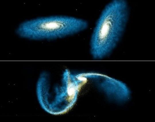
Matt Williams, Author at Universe Today

December 10, 2010May 16, 2016 by Matt Williams

What is the Coefficient of Friction?

Ever watch a car spin its wheels and notice all the smoke and tire marks it leaves behind? How about going down a slide? You might have noticed that if it were wet, you travelled farther than if the surface was dry. Ever wonder just how far you’d get if you tried to slide on wet concrete (don’t this, by the way!). Why is it that some surfaces are easy to slide across while others are just destined to stop you short? It comes down to a little thing known as friction, which is essentially the force that resists surfaces from sliding against each other. When it comes to measuring friction, the tool which scientists use is called the Coefficient of Friction or COH.

The COH is the value which describes the ratio of the force of friction between two bodies and the force pressing them together. They range from near zero to greater than one, depending on the types of materials used.For example, ice on steel has a low coefficient of friction, while rubber on pavement (i.e. car tires on the road) has a comparatively high one. In short, rougher surfaces tend to have higher effective values whereas smoother surfaces have lower due to the friction they generate when pressed together.

There are essentially two kind of coefficients; static and kinetic. The static coefficient of friction is the coefficient of friction that applies to objects that are motionless. The kinetic or sliding coefficient of friction is the coefficient of friction that applies to objects that are in motion.The coefficient of friction is not always the same for objects that are motionless and objects that are in motion; motionless objects often experience more friction than moving ones, requiring more force to put them in motion than to sustain them in motion.

Most dry materials in combination have friction coefficient values between 0.3 and 0.6. Values outside this range are rarer, but teflon, for example, can have a coefficient as low as 0.04. A value of zero would mean no friction at all, which is elusive at best, whereas a value above 1 would mean that the force required to slide an object along the surface is greater than the normal force of the surface on the object.

Mathematically, frictional force can be expressed asFf= ? N, where Ff = frictional force (N, lb), ? = static (?s) or kinetic (?k) frictional coefficient, N = normal force (N, lb).

We have written many articles about the coefficient of friction for Universe Today. Here’s an article about friction, and here’s an article about aerobraking.

If you’d like more info on the Friction, check out Hyperphysics, and here’s a link to Friction Games for Kids by Science Kids.

We’ve also recorded an entire episode of Astronomy Cast all about Gravity. Listen here, Episode 102: Gravity.

Sources:
http://en.wikipedia.org/wiki/Friction
http://www.engineeringtoolbox.com/friction-coefficients-d_778.html
http://www.thefreedictionary.com/coefficient+of+friction

December 4, 2010December 24, 2015 by Matt Williams

Chromatic Aberration

[/caption]

Some colours just can’t keep up with the others! Well, that’s probably the simplest way to put it. But when scientists talk about the characteristics of light, it would be more accurate to say that different colours of light propagate at different speeds, orhave different wavelengths, and therefore refract differently. A well-known example of this is the prism effect, where a beam of white light is broken into a rainbow of colours. The result of this is that when objects are viewed through a simple lens, light will refract (bends) at different angles, meaning that it will not image all in the same place. A distortion results in which “fringes” of color appear along the boundaries that separate dark and bright parts of the image. This effect, known as Chromatic Aberration, can be a real pain for astronomers, surveyors, photographers, or just about anyone who wants to view an object (or objects) through a lens and needs to do so clearly!

Sir Isaac Newton was the first to demonstrate this effect some two-hundred years ago when he discovered that light was composed of multiple wavelengths. These colours refract unevenly, with blue-appearing light refracting at shorter wavelengths and red-appearing light refracting at longer, with green refracting in the middle. Since that time, scientists, astronomers and opticians have come to identify two basic kinds of aberration. The first is axial (or longitudinal) where different wavelengths are focused at a different distance because the lens in unable to focus different colours in the same focal plane. The second is transverse (or lateral) aberration, where different wavelengths are focused at different positions in the focal plane and the effect is a sideward displacement of the image. In the former case, distortion occurs throughout the image whereas in the latter, distortion is absent from the centre but increases towards the edge.

There are many ways to remedy Chromatic Aberration. During the 17th century, telescopes had to be very long in order to correct for colour distortions. Sir Isaac Newton remedied this problem by creating the comparably compact, reflecting telescope in 1668 that used curved mirrors to get around this problem. The achromatic lens (or achromatic doublet) is another; a double lens that uses two kinds of glass that focuses all white light coming in at the same point on the other side of the lens. Many types of glass, known as low dispersion glasses, have been developed to reduce chromatic aberration, the most notable being glasses that contain fluorite.

The discovery of Chromatic Aberration and the development of corrective lenses were major steps in the development of the optical microscope, the telescope; which in turn was a boon for astronomers and biologist who were able to gain a greater understanding of the universe and the natural world as a result.

We have written many articles about chromatic aberration for Universe Today. Here’s an article about optical aberration, and here’s an article about achromatic lens.

If you’d like more info on Chromatic Aberration, check out Hyperphysics for a great article on chromatic aberration, and here’s a link to Wise Geek’s discussion about chromatic aberration.

We’ve also recorded an entire episode of Astronomy Cast all about Choosing and Using a Telescope. Listen here, Episode 33: Choosing and Using a Telescope.

Sources:
http://en.wikipedia.org/wiki/Chromatic_aberration
http://toothwalker.org/optics/chromatic.html
http://hyperphysics.phy-astr.gsu.edu/hbase/geoopt/aber2.html
http://www.yorku.ca/eye/chroaber.htm
http://www.yorku.ca/eye/achromat.htm

December 3, 2010December 24, 2015 by Matt Williams

Charles Law

[/caption]

For most people, the words “ideal gas” might conjure up the image of some kind of super fuel, perhaps a near-inexhaustible kind that creates zero air pollution! Sadly, this is not what is meant by ideal gas. In reality, an ideal gas is a theoretical gas composed of a set of randomly-moving, non-interacting point particles. At normal conditions such as standard temperature and pressure, most real gases such as air, nitrogen, oxygen, hydrogen, noble gases, and some heavier gases like carbon dioxide behave like an ideal gas and can be treated as such within reasonable tolerances. It is only when they are treated with higher temperatures and lower pressure that they deviate from this trend. Once they get into this territory, experimental gas laws, such as Charles’s Law, come into play.

Also known as the law of volumes, Charles’s Law is an experimental gas law which describes how gases tend to expand when heated. It was first published by French natural philosopher Joseph Louis Gay-Lussac in 1802, although he credited the discovery to unpublished work from the 1780s by Jacques Charles, hence the name. This law applies generally to all gases, and also to the vapours of volatile liquids if the temperature is more than a few degrees above the boiling point. Given the interest in hot air balloons at the time, it is certainly understandable why Gay-Lussac, Charles and other scientists around the globe were so interested in the relationship between volume, pressure and temperature when it came to gasses.

In lay terms, the law states that: at constant pressure, the volume of a given mass of an ideal gas increases or decreases by the same factor as its temperature on the absolute temperature scale (i.e. the gas expands as the temperature increases). This can be written as: V? T, where V is the volume of the gas; and T is the absolute temperature. In mathematical terms, the law can also be expressed as: V100 – V0 = kV0, where V100 is the volume occupied by a given sample of gas at 100 °C; V0 is the volume occupied by the same sample of gas at 0 °C; and k is a constant which is the same for all gases at constant pressure. Gay-Lussac’s value for k was ½.6666, remarkably close to the present-day value of ½.7315.

Combined with Boyle’s law, these laws make up what is known as the “Ideal Gas Law” which was first stated by ÉmileClapeyron in 1834.

We have written many articles about Charles’s Law for Universe Today. Here’s an article about the Combined Gas Law, and here’s an article about Boyle’s Law.

If you’d like more info on Charles’s Law, check out a discussion about Charles’s Law, and here’s a link to an article about Charles’s Law by the Glenn Research Center.

We’ve also recorded an episode of Astronomy Cast all about planet Earth. Listen here, Episode 51: Earth.

Sources:
http://en.wikipedia.org/wiki/Charles%27s_law
http://en.wikipedia.org/wiki/Ideal_gas
http://www.chm.davidson.edu/vce/gaslaws/charleslaw.html
http://www.grc.nasa.gov/WWW/K-12/airplane/glussac.html
http://en.wikipedia.org/wiki/Ideal_gas_law

November 19, 2010January 16, 2017 by Matt Williams

What is Planck Time?

What is the smallest unit of time you can conceive? A second? A millisecond? Hard to say seeing as how time is relative. Under the right circumstances, hours can fly by and seconds can feel like a lifetime. But unfortunately for physicists, time is not something that can be dealt with so philosophically. And since they deal with cosmological forces both infinitesimally large and small, they need units that can objectively measure them. When it comes to dealing with the small, Planck Time is the measurement of choice. Named after German physicist Max Planck, the founder of quantum theory, a unit of Planck time is the time it takes for light to travel, in a vacuum, a single unit of Planck length. Taken together, they part of the larger system of natural units known as Planck units.

Originally proposed in 1899 by German physicist Max Planck, Planck units are physical units of measurement defined exclusively in terms of five universal physical constants. These are the Gravitational constant (G), the Reduced Planck constant (h), the speed of light in a vacuum (c), the Coulomb constant 1/4??0 (ke or k), and Boltzmann’s constant (kB, sometimes k). Each of these constants can be associated with at least one fundamental physical theory: c with special relativity, G with general relativity and Newtonian gravity, ? with quantum mechanics, ?0 with electrostatics, and kB with statistical mechanics and thermodynamics. They were invented as a means of simplifying the particular algebraic expressions appearing in theoretical physics, especially in quantum mechanics.

Ultimately, Planck time is derived from the field of mathematical physics known as dimensional analysis, which studies units of measurement and physical constants. The Planck time is the unique combination of the gravitational constant G, the relativity constant c, and the quantum constant h, to produce a constant with units of time. They are often semi-humorously referred to by physicists as “God’s units” because eliminate anthropocentric arbitrariness from the system of units, unlike the meter and second, which exist for purely historical reasons and are not derived from nature. Some challenges to Planck’s Time have been mounted. For example, in 2003 during the analysis of the Hubble Space Telescope Deep Field images, some scientists speculated that where there are space-time fluctuations on the Planck scale, images of extremely distant objects should be blurry. The Hubble images, they claimed, were too sharp for this to be the case. Other scientists disagreed with this assumption however, with some saying the fluctuations would be too small to be observable, others saying that the speculated blurring effect that was expected was off by a very large magnitude.

A unit of Planck Time can be expressed as follows:

Planck Time

We have written many articles about Planck Time for Universe Today. Here’s an article about the Big Bang Theory, and here’s an article about astronomical units.

If you’d like more info on the Planck Time, check out Wikipedia, and here’s a link to Physics and Astronomy Online.

We’ve also recorded a Question Show all about Black Hole Time. Listen here, Question Show: Galileoscope, Black Hole and What Exactly is Energy?.

Sources:
http://en.wikipedia.org/wiki/Planck_time
http://en.wikipedia.org/wiki/Max_Planck
http://en.wikipedia.org/wiki/Planck_units
http://scienceworld.wolfram.com/physics/PlanckTime.html
http://en.wikipedia.org/wiki/Dimensional_analysis

November 18, 2010April 26, 2016 by Matt Williams

North American Plate

[/caption]

Oftentimes when we think of the Earth, we tend to think of stable landmasses that are surrounded by vast oceans. It’s easy for us to forget that the Earth is still very much a work in a progress, that its foundations are mobile slabs of rock, known as plates, which are constantly on the move and shuffling back and forth. In our next of the woods, aka. North American, we inhabit what is appropriately named the North American Plate, the tectonic boundary that covers most of North America, Greenland, Cuba, Bahamas, and parts of Siberia and Iceland. It extends eastward to the Mid-Atlantic Ridge and westward to the Chersky Range in eastern Siberia. It is composed of two types of lithosphere: the upper crust (where the continental land masses reside) and the thinner oceanic crust.

As one of the Earth’s original continents, the North American Plate started forming some three billion years ago when the planet was much hotter and mantle convection much more vigorous. Roughly two billions years ago, the Earth cooled and these old floating pieces of the lithosphere, called cratons, stopped growing. Since that time, the plates have been moving back and forth across the globe, their cratons colliding to form the continents that we know and recognize today. Beginning in the Cambrian period, over five hundred million years ago, the cratons of Laurentia and Siberia broke off from the main landmass of Pangaea, which thereafter would be known as Gondwana. By the late Mezosoic era (circa two hundred million years ago) the Laurentian and Eurasian cratons combined to form the supercontinent of Laurasia. Since that time, the separation of the North American and Eurasian plates has led to the separation of the North America from Asia. As the North American plate drifted west, the landmasses of Iceland and Greenland broke off in the east while in the west, it collided with the Eurasian plate again, adding the landmass of Siberia to East Asia.

In terms of what makes the plates move across the Earth, a number of theories coexist. One theory is what is known as the “conveyor belt” principle, where the Earth’s lithosphere has a higher strength and lower density than the underlying asthenosphere and lateral density variations in the mantle result in the slow drifting motion of the plates, resulting in collisions and subduction zones. One of the main points of the theory is that the amount of surface of the plates that disappear through subduction along the boundaries where they collide is more or less equal to the new crust that is formed along the margins where they are drifting apart. In this way, the total surface of the Globe remains the same. A different explanation lies in different forces generated by the rotation of the Globe and tidal forces of the Sun and the Moon. A final theory which predates the Plate Tectonics “paradigm”, has it that a gradual shrinking (contraction) or gradual expansion of the Globe is responsible.

We have written many articles about the North American Plate for Universe Today. Here’s an article about the continental plate, and here’s an article about the plate tectonics theory.

If you’d like more info on Earth, check out NASA’s Solar System Exploration Guide on Earth. And here’s a link to NASA’s Earth Observatory.

We’ve also recorded related episodes of Astronomy Cast about Plate Tectonics. Listen here, Episode 142: Plate Tectonics.

Sources:
http://en.wikipedia.org/wiki/North_American_Plate
http://en.wikipedia.org/wiki/Plate_tectonics
http://www.platetectonics.com/book/page_5.asp
http://www.uwgb.edu/dutchs/GeolColBk/NAmerPlate.HTM
http://en.wikipedia.org/wiki/Mantle_convection
http://en.wikipedia.org/wiki/Craton
http://en.wikipedia.org/wiki/Laurasia

November 17, 2010December 24, 2015 by Matt Williams

Tertiary Period

[/caption]

When it comes to the geological timeline, there are several periods that scientists and biologists recognize as being of extreme importance to the development of life on Earth. There’s the Hadean period, which began with the creation of the Earth and was marked by the formations of the oceans and atmosphere. Or the Cambrian period, when the massive continent of Pangaea broke up and allowed for the explosion of life which led to the development of all modern Phyla. But when it comes to us mammals, perhaps the most important period was the one known as the Tertiary Period. This period began 65 million years ago and ended roughly 1.8 million years ago and bore witness to some major geological, biological and climatological events. This included the current configuration of the continents, the cooling of global temperatures, and the rise of mammals as the planet’s dominant vertebrates. It followed the Cretaceous period and was superseded by the Quaternary.

In terms of major events, the Tertiary period began with the demise of the non-avian dinosaurs in the Cretaceous–Tertiary extinction event, at the start of the Cenozoic era, and lasted to the beginning of the most recent Ice Age at the end of the Pliocene epoch. In terms of geology, there was a great deal of tectonic activity that continued from the previous era, culminating in the splitting of Gondwana and the collision of the Indian landmass with the Eurasian plate. This led to the formation of the Himalayas, the gradual creation of the continent of Australia (a haven for the non-placental, marsupial mammals), the separation South America from West Africa and its connection to North America, and Antarctica taking its current position below the South Pole. In terms of climate, the period was marked by widespread cooling, beginning in the Paleocene with tropical-to-moderate worldwide temperatures and ending before the first extensive glaciation at the start of the Quaternary.

In terms of species evolution, this period was of extreme importance to modern life. By the beginning of the period, mammals replaced reptiles as the dominant vertebrates on the planet. In addition, all non-avian dinosaurs (referring to terrestrial dinosaurs and not their avian descendants) had all become extinct by the beginning of this period. Modern types of birds, reptiles, amphibians, fish, and invertebrates were already numerous at the beginning of this period but also continued to appeared early on, and many modern families of flowering plants evolved. And last, but certainly not least (at least for us human folk), the earliest recognizable hominid relatives of humans appeared. One striking example of this is the Proconsul Primate, a tree-dwelling Primate that existed from roughly 23 to 17 million years ago and who’s fossilized remains have been found today in modern Kenya, Uganda and other East African locales.

We have written many articles about Tertiary Period for Universe Today. Here’s an article about the Quaternary Period, and here’s an article about the asteroid extinction theory.

If you’d like more info on the Tertiary Period, check out the USGS Geologic Time Scale, and here’s a link to another article about the Tertiary Period.

We’ve also recorded an episode of Astronomy Cast all about planet Earth. Listen here, Episode 51: Earth.

Sources:
http://en.wikipedia.org/wiki/Tertiary
http://en.wikipedia.org/wiki/Cretaceous%E2%80%93Tertiary_extinction_event
http://en.wikipedia.org/wiki/Gondwana#Cenozoic
http://en.wikipedia.org/wiki/Proconsul_%28genus%29
http://en.wikipedia.org/wiki/Dinosaur

November 17, 2010December 24, 2015 by Matt Williams

Super Magnets

Permanent Magnet — Super Magnets, the strongest type of permanent magnets

[/caption]

Magnets are not only a source of endless fun – for children and children of all ages! They also happen to have endless industrial applications. But when it comes to the high-tech industry, the people who rely on magnetic materials to build appliances, electronics, or even spaceships, only one type of magnet will do. These are known as Rare Earth or Super Magnets, the kind that are used in MRI machines, computer hard drives, electric and hybrid motors, audio speakers, electric guitars, and race car engines. In spite of their name, the elements used to make super magnets are actually quite common, but were rarely found in large enough quantities to be considered economically viable. However, since the 90’s these magnets have become cheap and widely available, and are even being considered for additional processes.

The term super magnet is a broad term and encompasses several families of rare-earth magnets that include seventeen elements in the periodic table; namely scandium, yttrium, and the fifteen lanthanides. First developed in the 1970’s and 80’s, super magnets are the strongest type of permanent magnets ever made, are ferromagnetic, meaning that like iron they can be magnetized, and have Curie temperatures that are below room temperature. This means that in their pure form, their magnetism only appears at low temperatures. However, since they can form compounds with transition metals such as iron, nickel, and cobalt, metals that have Curie temperatures well above room temperature, they can be used effectively at higher temperatures as well. The main advantage they have over conventional magnets is that their greater strength allows for smaller, lighter magnets to be used, ones that can do the same job but take up less space and require less material.

Super magnets can be broken down into two categories. First, there is the neodymium magnet, which is made from an alloy of neodymium, iron, and boron to form the Nd2Fe14B tetragonal crystalline structure. This material is currently the strongest known type of permanent magnet and was developed in the 1980’s. It is typically used in the construction of head actuators in computer hard drives and has many electronic applications, such as electric motors, appliances, and magnetic resonance imaging (MRI). The second type of super magnet is the samarium-cobalt variety, an alloy of samarium and cobalt with the chemical formula of SmCo5. This second-strongest type of rare Earth magnet is also used in electronic motors, turbomachinery, and because of its high temperature range tolerance may also have many applications for space travel, such as cryogenics and heat resistant machinery.

We have written many articles about magnets for Universe Today. Here’s an article about where to buy magnets, and here’s an article about what magnets are made of.

If you’d like more info on Super Magnets, check out Rare Earth Magnetics Homepage, and here’s a link to Wikipedia: Rare Earth Magnets.

We’ve also recorded an entire episode of Astronomy Cast all about Magnetism. Listen here, Episode 42: Magnetism Everywhere.

Sources:
http://en.wikipedia.org/wiki/Rare-earth_magnet
http://en.wikipedia.org/wiki/Magnet
http://en.wikipedia.org/wiki/Samarium-cobalt_magnet
http://en.wikipedia.org/wiki/Neodymium_magnet
http://www.newton.dep.anl.gov/askasci/phy99/phy99010.htm

November 12, 2010August 26, 2021 by Matt Williams

How Much Does the Earth Weigh?

Winter Solstice — Earth as viewed from the cabin of the Apollo 11 spacecraft. Credit: NASA

Earth is, by any reckoning, a pretty big place. Ever since humanity first began the process of exploring, philosophers and scholars have sought to understand its exact dimensions. In addition to wanting to quantify its diameter, circumference, and surface area, they have also sought to understand just how much weight it packs on.

In terms of mass, Earth is also a pretty big customer. Compared to the other bodies of the Solar System, it is the largest and densest of the rocky planets. And over the course of the past few centuries, our methods for determining its mass have improved – leading to the current estimate of 5.9736×10²⁴kg (1.31668×10²⁵ lbs).

Size and Composition:

With a mean radius of 6,371.0 km (3,958.8 mi), Earth is the largest terrestrial planet in our Solar System. This means that it is composed primarily of silicate rock and metals, which are differentiated between a solid inner core, an outer core of molten metal, and a silicate mantle and crust made of silicate material.

This cutaway of planet Earth shows the familiar exterior of air, water and land as well as the interior: from the mantle down to the outer and inner cores. Currents in hot, liquid iron-nickel in the outer core create our planet's protective but fluctuating magnetic field. Credit: Kelvinsong / Wikipedia — *This cutaway of planet Earth shows the familiar exterior of air, water and land as well as the interior: from the mantle down to the outer and inner cores. Credit: Kelvinsong / Wikipedia*

Earth is composed approximately of 32% iron, 30% oxygen, 15% silicon, 14% magnesium, 3% sulfur, 2% nickel, 1.5% calcium, and 1.4% aluminum, with the remaining made up of trace elements. Meanwhile, the core region is primarily composed of iron (88.8%), with smaller amounts of nickel (5.8%), sulfur (4.5%), and less than 1% trace elements.

Mass and Density:

Earth is also the densest planet in the Solar System, with a mean density of 5.514 g/cm³ (0.1992 lbs/cu in). Between its size, composition, and the distribution of its matter, the Earth has a mass of 5.9736×10²⁴kg (~5.97 billion trillion metric tons) or 1.31668×10²⁵ lbs (6.585 billion trillion tons).

But since the Earth’s density is not even throughout – i.e. it is denser towards the core than it is at its outer layers – its mass is also not evenly distributed. In fact, the density of the inner core (at 12.8 to 13.1 g/cm³; 0.4624293 lbs/cu in), while the density of the crust is just 2.2–2.9 g/cm³ (0.079 – 0.1 lbs/cu in).

*The layers of the Earth, a differentiated planetary body. Credit: Wikipedia Commons/Surachit*

This overall mass and density are also what causes Earth to have a gravitational pull equivalent to 9.8 m/s² (32.18 ft/s²), which is defined as 1 g.

History of Study:

Modern scientists discerned what the mass of the Earth was by studying how things fall towards it. Gravity is created by mass, so the more mass an object has, the more gravity it will pull with. If you can calculate how an object is being accelerated by the gravity of an object, like Earth, you can determine its mass.

In fact, astronomers didn’t accurately know the mass of Mercury or Venus until they finally put spacecraft into orbit around them. They had rough estimates, but once there were orbiting spacecraft, they could make the final mass calculations. We know the mass of Pluto because we can calculate the orbit of its moon Charon.

*The Geoid 2005 model, which was based on data of two satellites (CHAMP and GRACE) plus surface data. Credit: GFZ*

And by studying other planets in our Solar System, scientists have had a chance to improve the methods and instruments used to study Earth. From all of this comparative analysis, we have learned that Earth outstrips Mars, Venus, and Mercury in terms of size, and all other planets in the Solar System in terms of density.

In short, the saying “it’s a small world” is complete rubbish!

We have written many articles about Earth for Universe Today. Here’s Ten Interesting Facts About Earth, What is the Diameter of the Earth?, How Strong is the Force of Gravity on Earth?, What is the Rotation of the Earth?

If you’d like more info on Earth, check out NASA’s Solar System Exploration Guide on Earth. And here’s a link to NASA’s Earth Observatory.

We’ve also recorded an episode of Astronomy Cast all about planet Earth. Listen here, Episode 51: Earth.

Sources:

November 11, 2010December 24, 2015 by Matt Williams

Subatomic Particles

[/caption]

Not long ago, scientists believed that the smallest part of matter was the atom; the indivisible, indestructible, base unit of all things. However, it was not long before scientists began to encounter problems with this model, problems arising out of the study of radiation, the laws of thermodynamics, and electrical charges. All of these problems forced them to reconsider their previous assumptions about the atom being the smallest unit of matter and to postulate that atoms themselves were made up of a variety of particles, each of which had a particular charge, function, or “flavor”. These they began to refer to as Subatomic Particles, which are now believed to be the smallest units of matter, ones that composenucleons and atoms.

Whereas protons, neutrons and electrons have always been considered to be the fundamental particles of an atom, recent discoveries using atomic accelerators have shown that there are actually twelve different kinds of elementary subatomic particles, and that protons and neutrons are actually made up of smaller subatomic particles. These twelve particles are divided into two categories, known as Leptons and Quarks. There are six different kinds, or “flavors”, of quarks (named because of their unusual behavior). These include up, down, charm, strange, top, and bottom quark, each of which possesses a charge that is expressed as a fraction (+2/3 for up, top and charm,-1/3 for down, bottom and strange) and have variable masses. There are also six different types of Leptons, which include Electrons, Muons, Taus, Electron Neutrinos, Muon Neutrinos, and Tau Neutrinos. Whereas electrons and Muons both have a negative charge of -1 (Muons having greater mass), Neutrinos have no charge and are extremely difficult to detect.

In addition to elementary particles, composite particles are another category of subatomic particles. Whereas elementary particles are not made up of other particles, composite particlesare bound states of two or more elementary particles, such as protons or atomic nuclei. For example, a proton is made of two Up quarks and one Down quark, while the atomic nucleus of helium-4 is composed of two protons and two neutrons.In addition, there are also the subatomic particles that fall under the heading of Gauge Bosons, which were identified using the same methods as Leptons and Quarks. These are classified as “force carriers”, i.e. particles that act as carriers for the fundamental forces of nature. These include photons that are associated with electromagnetism, gravitons that are associated with gravity, the three W and Z bosons of weak nuclear forces, and the eight gluons of strong nuclear forces. Scientists also predict the existence of several more, what they refer to as “hypothetical” particles, so the list is expected to grow.

Today, there are literally hundreds of known subatomic particles, most of which were either the result of cosmic rays interacting with matter or particle accelerator experiments.

We have written many articles about the subatomic particles for Universe Today. Here’s an article about the atomic nucleus, and here’s an article about the atomic theory.

If you’d like more info on the Atom, check out the Background on Atoms, and here’s a link to the NASA’s Understanding the Atom Page.

We’ve also recorded an entire episode of Astronomy Cast all about the Composition of the Atom. Listen here, Episode 164: Inside the Atom.

Sources:
http://en.wikipedia.org/wiki/Subatomic_particle
http://en.wikipedia.org/wiki/Nucleon
http://www.school-for-champions.com/science/subatomic.htm
http://en.wikipedia.org/wiki/Gauge_boson
http://en.wikipedia.org/wiki/List_of_particles

November 11, 2010December 24, 2015 by Matt Williams

Star Cluster

[/caption]

There are few things in astronomy more awe inspiring and spellbinding than the birth of a star. Even though we now understand how they are formed, the sheer magnitude of it is still enough to stir the imagination of even the most schooled and cynical academics. Still, there is some degree of guesswork and chance when it comes to where stars will be born and what kind of stars they will become. For example, while some stars are single field stars (like our Sun), others form in groups of two (binary) or more, sometimes much more. This is what is known as a Star Cluster, by definition, a group of stars that share a common origin and are gravitationally bound for some length of time.

Thereare two basic categories of star clusters: Globular and Open (aka. Galactic) star clusters. Globular clusters are roughly spherical groupings of stars that range from 10,000 to several million stars packed into regions ranging from 10 to 30 light years across. They commonly consist of very old Population II stars – which are just a few hundred million years younger than the universe itself – and are mostly yellow and red. Open clusters, on the other hand, are very different. Unlike the spherically distributed globulars, open clusters are confined to the galactic plane and are almost always found within the spiral arms of galaxies. They are generally made up of young stars, up to a few tens of millions of years old, with a few rare exceptions that are as old as a few billion years. Open clusters also contain only a few hundred members within a region of up to about 30 light-years. Being much less densely populated than globular clusters, they are much less tightly gravitationally bound, and over time, will become disrupted by the gravity of giant molecular clouds and other clusters.

Star clusters are particularly useful to astronomers as they provide a way to study and model stellar evolution and ages. By estimating the age of globular clusters, scientists were able to get a more accurate picture of how old the universe is, putting it at roughly 13 billion years of age. In addition, the location of star clusters and galaxies is believed to be a good indication of the physics of the early universe. This is based on aspects of the Big Bang theory where it is believed that immediately after the creation event, following a period of relatively homogenous distribution; cosmic matter slowly gravitated to areas of higher concentration. In this way, star clusters and the position of galaxies provide an indication of where matter was more densely distributed when the universe was still young.

Some popular examples of star clusters, many of which are visible to the naked eye, include Pleiades, Hyades, the Beehive Cluster and the star nursery within the Orion Nebula.

We have written many articles about star cluster for Universe Today. Here’s an article about a massive star cluster discovered, and here are some amazing star cluster wallpapers.

If you’d like more information on stars, check out Hubblesite’s News Releases about Stars, and here’s the stars and galaxies homepage.

We’ve done many episodes of Astronomy Cast about stars. Listen here, Episode 12: Where Do Baby Stars Come From?

Sources:
http://en.wikipedia.org/wiki/Star_cluster
http://universe-review.ca/F06-star-cluster.htm
http://outreach.atnf.csiro.au/education/senior/astrophysics/stellarevolution_clusters.html
http://www.sciencedaily.com/articles/s/star_cluster.htm
http://en.wikipedia.org/wiki/Stellar_populations#Populations_III.2C_II.2C_and_I
http://www.sciencedaily.com/articles/g/galaxy_formation_and_evolution.htm