Matt Williams, Author at Universe Today

September 1, 2016September 6, 2016 by Matt Williams

What is the Speed of Light?

Artist's impression of a spaceship making the jump to "light speed". Credit: NASA/Glenn Research Center

Since ancient times, philosophers and scholars have sought to understand light. In addition to trying to discern its basic properties (i.e. what is it made of – particle or wave, etc.) they have also sought to make finite measurements of how fast it travels. Since the late-17th century, scientists have been doing just that, and with increasing accuracy.

In so doing, they have gained a better understanding of light’s mechanics and the important role it plays in physics, astronomy and cosmology. Put simply, light moves at incredible speeds and is the fastest moving thing in the Universe. Its speed is considered a constant and an unbreakable barrier, and is used as a means of measuring distance. But just how fast does it travel?

Speed of Light (c):

Light travels at a constant speed of 1,079,252,848.8 (1.07 billion) km per hour. That works out to 299,792,458 m/s, or about 670,616,629 mph (miles per hour). To put that in perspective, if you could travel at the speed of light, you would be able to circumnavigate the globe approximately seven and a half times in one second. Meanwhile, a person flying at an average speed of about 800 km/h (500 mph), would take over 50 hours to circle the planet just once.

Illustration showing the distance between Earth and the Sun. Credit: LucasVB/Public Domain — *Illustration showing the distance light travels between the Earth and the Sun. Credit: LucasVB/Public Domain*

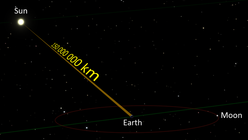
To put that into an astronomical perspective, the average distance from the Earth to the Moon is 384,398.25 km (238,854 miles ). So light crosses that distance in about a second. Meanwhile, the average distance from the Sun to the Earth is ~149,597,886 km (92,955,817 miles), which means that light only takes about 8 minutes to make that journey.

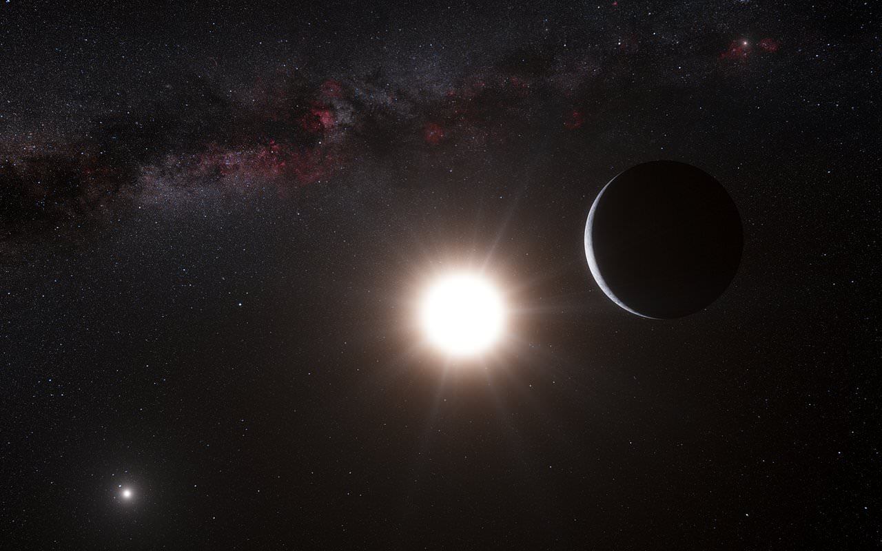
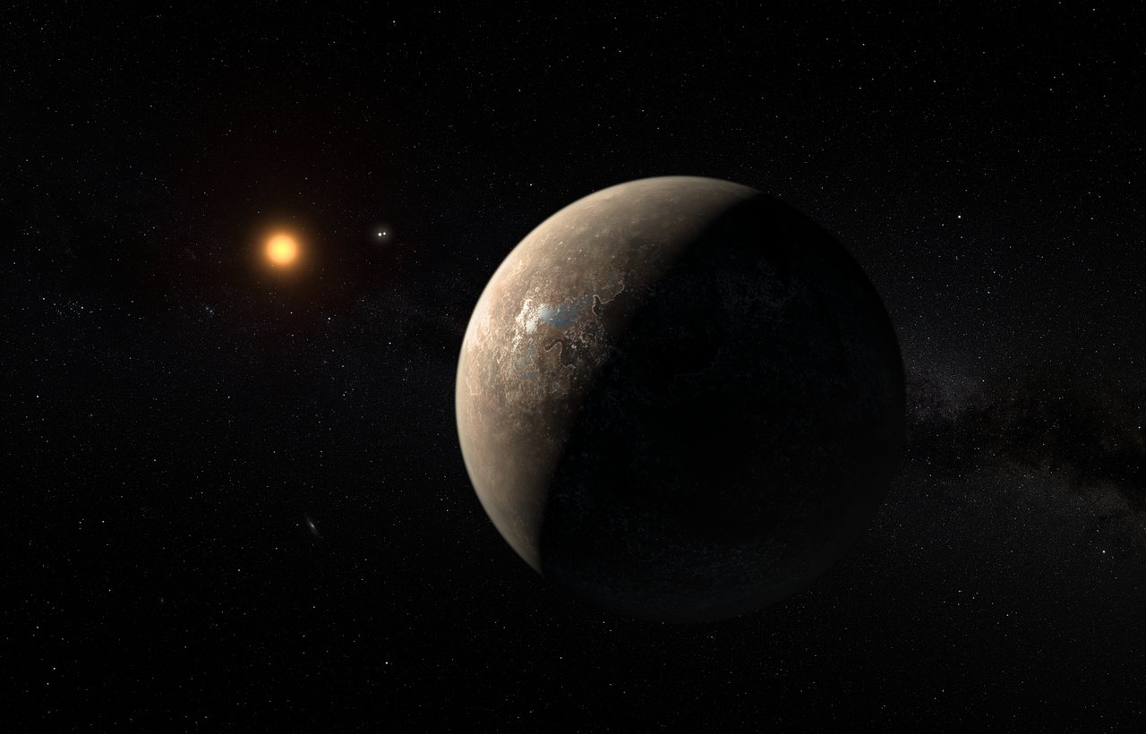
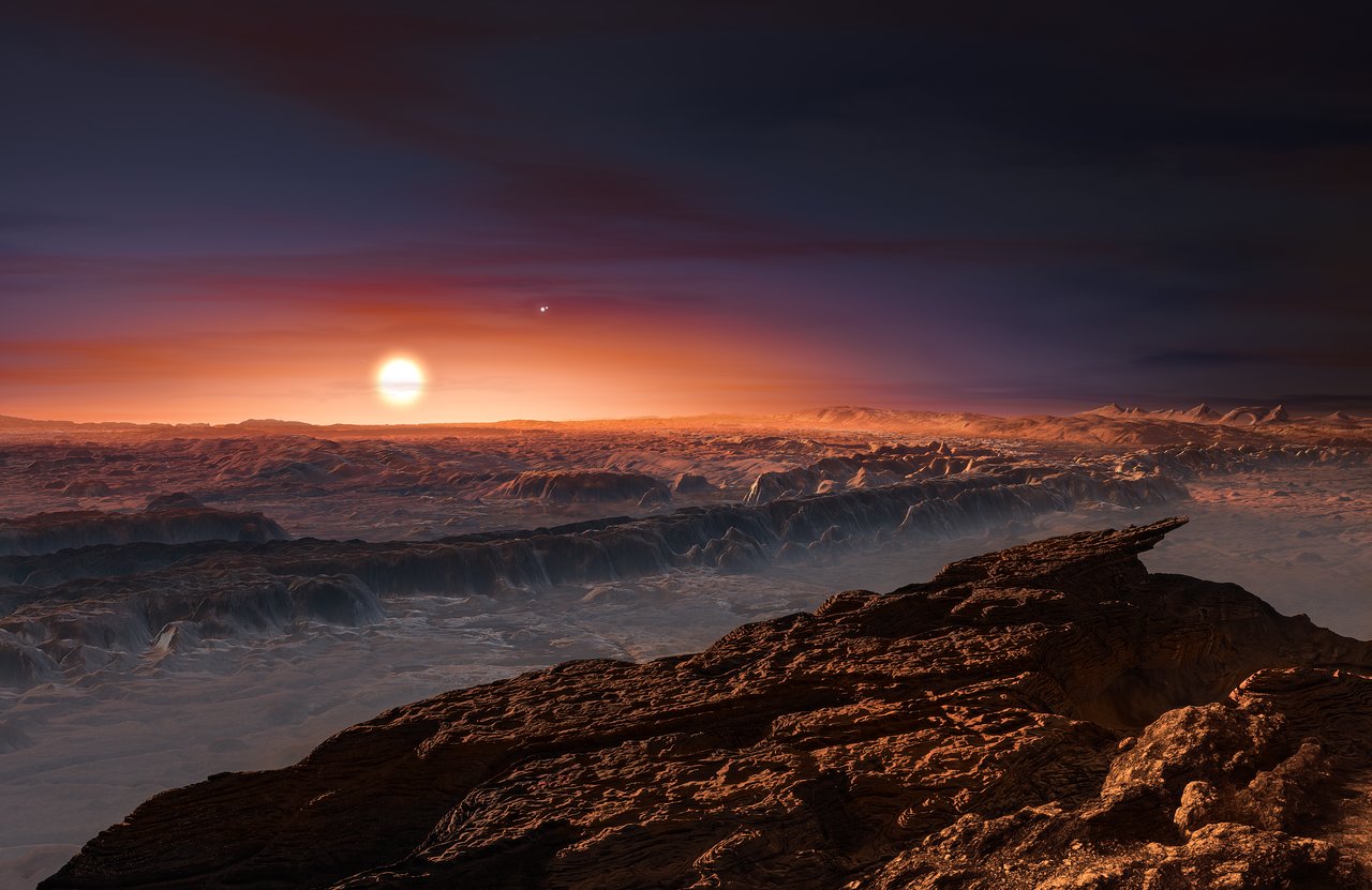
Little wonder then why the speed of light is the metric used to determine astronomical distances. When we say a star like Proxima Centauri is 4.25 light years away, we are saying that it would take – traveling at a constant speed of 1.07 billion km per hour (670,616,629 mph) – about 4 years and 3 months to get there. But just how did we arrive at this highly specific measurement for “light-speed”?

History of Study:

Until the 17th century, scholars were unsure whether light traveled at a finite speed or instantaneously. From the days of the ancient Greeks to medieval Islamic scholars and scientists of the early modern period, the debate went back and forth. It was not until the work of Danish astronomer Øle Rømer (1644-1710) that the first quantitative measurement was made.

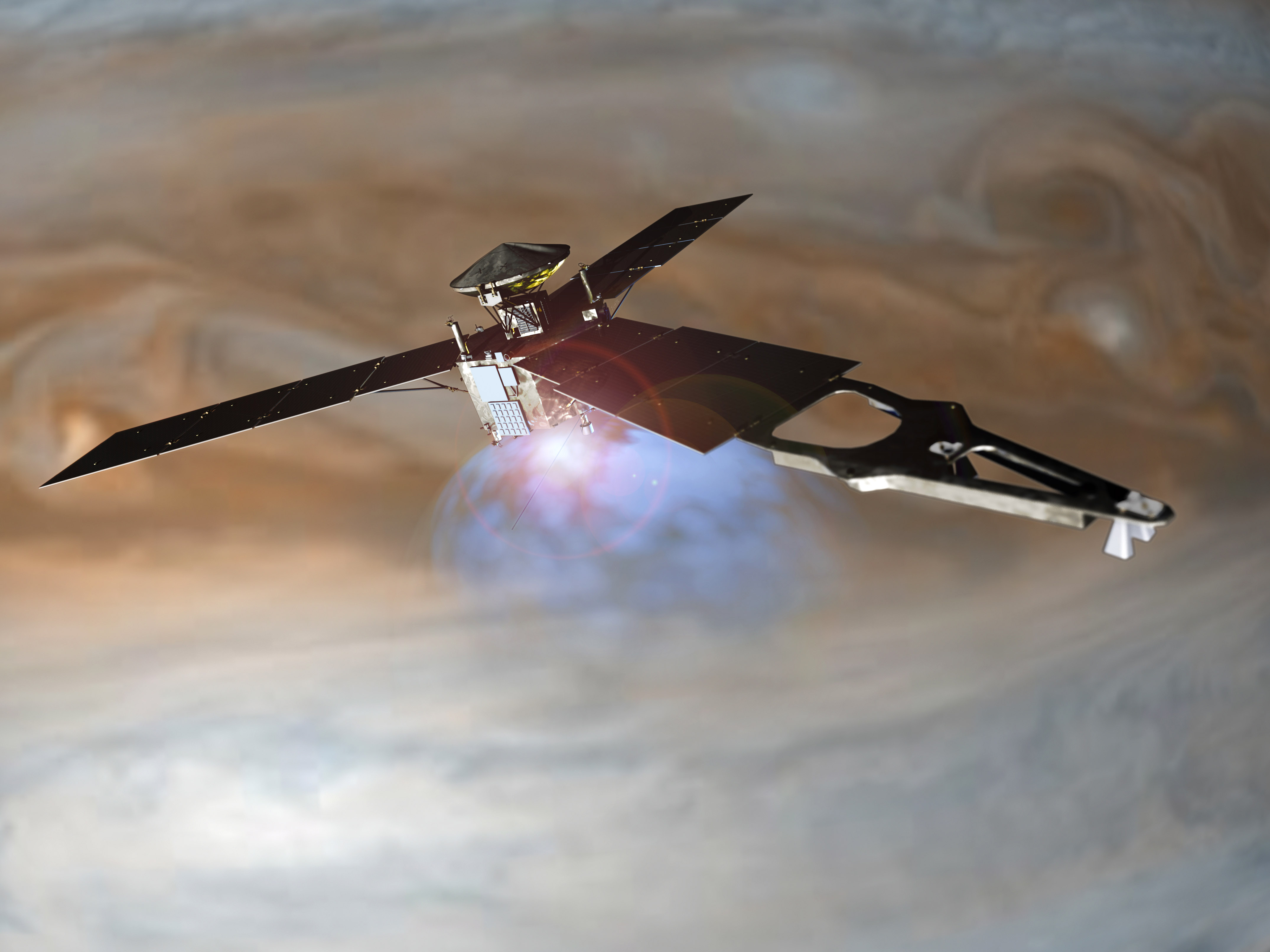
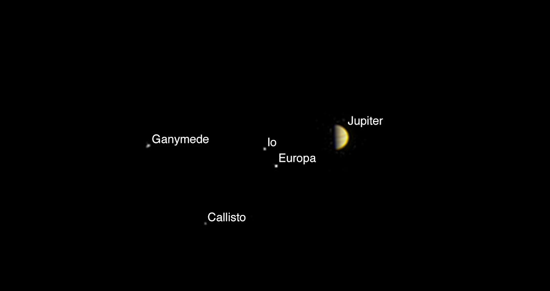
In 1676, Rømer observed that the periods of Jupiter’s innermost moon Io appeared to be shorter when the Earth was approaching Jupiter than when it was receding from it. From this, he concluded that light travels at a finite speed, and estimated that it takes about 22 minutes to cross the diameter of Earth’s orbit.

Prof. Albert Einstein uses the blackboard as he delivers the 11th Josiah Willard Gibbs lecture at the meeting of the American Association for the Advancement of Science in the auditorium of the Carnegie Institue of Technology Little Theater at Pittsburgh, Pa., on Dec. 28, 1934. Using three symbols, for matter, energy and the speed of light respectively, Einstein offers additional proof of a theorem propounded by him in 1905 that matter and energy are the same thing in different forms. (AP Photo) — Prof. Albert Einstein delivering the 11th Josiah Willard Gibbs lecture at the Carnegie Institute of Technology on Dec. 28th, 1934, where he expounded on his theory of how matter and energy are the same thing in different forms. Credit: AP Photo

Christiaan Huygens used this estimate and combined it with an estimate of the diameter of the Earth’s orbit to obtain an estimate of 220,000 km/s. Isaac Newton also spoke about Rømer’s calculations in his seminal work Opticks (1706). Adjusting for the distance between the Earth and the Sun, he calculated that it would take light seven or eight minutes to travel from one to the other. In both cases, they were off by a relatively small margin.

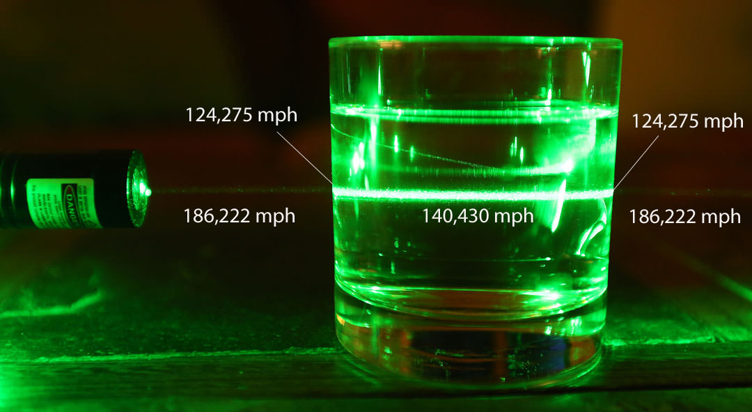
Later measurements made by French physicists Hippolyte Fizeau (1819 – 1896) and Léon Foucault (1819 – 1868) refined these measurements further – resulting in a value of 315,000 km/s (192,625 mi/s). And by the latter half of the 19th century, scientists became aware of the connection between light and electromagnetism.

This was accomplished by physicists measuring electromagnetic and electrostatic charges, who then found that the numerical value was very close to the speed of light (as measured by Fizeau). Based on his own work, which showed that electromagnetic waves propagate in empty space, German physicist Wilhelm Eduard Weber proposed that light was an electromagnetic wave.

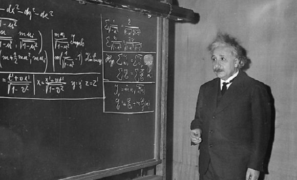
The next great breakthrough came during the early 20th century/ In his 1905 paper, titled “On the Electrodynamics of Moving Bodies”, Albert Einstein asserted that the speed of light in a vacuum, measured by a non-accelerating observer, is the same in all inertial reference frames and independent of the motion of the source or observer.

A laser shining through a glass of water demonstrates how many changes in speed it undergoes - from 186,222 mph in air to 124,275 mph through the glass. It speeds up again to 140,430 mph in water, slows again through glass and then speeds up again when leaving the glass and continuing through the air. Credit: Bob King — *A laser shining through a glass of water demonstrates how many changes in speed (in mph) it undergoes as it passes from air, to glass, to water, and back again. Credit: Bob King*

Using this and Galileo’s principle of relativity as a basis, Einstein derived the Theory of Special Relativity, in which the speed of light in vacuum (c) was a fundamental constant. Prior to this, the working consensus among scientists held that space was filled with a “luminiferous aether” that was responsible for its propagation – i.e. that light traveling through a moving medium would be dragged along by the medium.

This in turn meant that the measured speed of the light would be a simple sum of its speed through the medium plus the speed of that medium. However, Einstein’s theory effectively made the concept of the stationary aether useless and revolutionized the concepts of space and time.

Not only did it advance the idea that the speed of light is the same in all inertial reference frames, it also introduced the idea that major changes occur when things move close the speed of light. These include the time-space frame of a moving body appearing to slow down and contract in the direction of motion when measured in the frame of the observer (i.e. time dilation, where time slows as the speed of light approaches).

His observations also reconciled Maxwell’s equations for electricity and magnetism with the laws of mechanics, simplified the mathematical calculations by doing away with extraneous explanations used by other scientists, and accorded with the directly observed speed of light.

During the second half of the 20th century, increasingly accurate measurements using laser inferometers and cavity resonance techniques would further refine estimates of the speed of light. By 1972, a group at the US National Bureau of Standards in Boulder, Colorado, used the laser inferometer technique to get the currently-recognized value of 299,792,458 m/s.

Role in Modern Astrophysics:

Einstein’s theory that the speed of light in vacuum is independent of the motion of the source and the inertial reference frame of the observer has since been consistently confirmed by many experiments. It also sets an upper limit on the speeds at which all massless particles and waves (which includes light) can travel in a vacuum.

One of the outgrowths of this is that cosmologists now treat space and time as a single, unified structure known as spacetime – in which the speed of light can be used to define values for both (i.e. “lightyears”, “light minutes”, and “light seconds”). The measurement of the speed of light has also become a major factor when determining the rate of cosmic expansion.

Beginning in the 1920’s with observations of Lemaitre and Hubble, scientists and astronomers became aware that the Universe is expanding from a point of origin. Hubble also observed that the farther away a galaxy is, the faster it appears to be moving. In what is now referred to as the Hubble Parameter, the speed at which the Universe is expanding is calculated to 68 km/s per megaparsec.

This phenomena, which has been theorized to mean that some galaxies could actually be moving faster than the speed of light, may place a limit on what is observable in our Universe. Essentially, galaxies traveling faster than the speed of light would cross a “cosmological event horizon”, where they are no longer visible to us.

Also, by the 1990’s, redshift measurements of distant galaxies showed that the expansion of the Universe has been accelerating for the past few billion years. This has led to theories like “Dark Energy“, where an unseen force is driving the expansion of space itself instead of objects moving through it (thus not placing constraints on the speed of light or violating relativity).

Along with special and general relativity, the modern value of the speed of light in a vacuum has gone on to inform cosmology, quantum physics, and the Standard Model of particle physics. It remains a constant when talking about the upper limit at which massless particles can travel, and remains an unachievable barrier for particles that have mass.

Perhaps, someday, we will find a way to exceed the speed of light. While we have no practical ideas for how this might happen, the smart money seems to be on technologies that will allow us to circumvent the laws of spacetime, either by creating warp bubbles (aka. the Alcubierre Warp Drive), or tunneling through it (aka. wormholes).

Until that time, we will just have to be satisfied with the Universe we can see, and to stick to exploring the part of it that is reachable using conventional methods.

We have written many articles about the speed of light for Universe Today. Here’s How Fast is the Speed of Light?, How are Galaxies Moving Away Faster than Light?, How Can Space Travel Faster than the Speed of Light?, and Breaking the Speed of Light.

Here’s a cool calculator that lets you convert many different units for the speed of light, and here’s a relativity calculator, in case you wanted to travel nearly the speed of light.

Astronomy Cast also has an episode that addresses questions about the speed of light – Questions Show: Relativity, Relativity, and more Relativity.

Sources:

August 31, 2016May 5, 2019 by Matt Williams

On The Origin Of Phobos’ Groovy Mystery

Mars’ natural satellites – Phobos and Deimos – have been a mystery since they were first discovered. While it is widely believed that they are former asteroids that were captured by Mars’ gravity, this remains unproven. And while some of Phobos’ surface features are known to be the result of Mars’ gravity, the origin of its linear grooves and crater chains (catenae) have remained unknown.

But thanks to a new study by Erik Asphaug of Arizona State University and Michael Nayak from the University of California, we may be closer to understanding how Phobos’ got its “groovy” surface. In short, they believe that re-accretion is the answer, where all the material that was ejected when meteors impacted the moon eventually returned to strike the surface again.

Naturally, Phobos’ mysteries extend beyond its origin and surface features. For instance, despite being much more massive than its counterpart Deimos, it orbits Mars at a much closer distance (9,300 km compared to over 23,000 km). It’s density measurements have also indicated that the moon is not composed of solid rock, and it is known to be significantly porous.

(a) Spacecraft image of Phobos (photo credit: ESA/Mars Express) showing the observed catena of interest (red arrows); (b) reimpact map for a primary impact at Grildrig, azimuth ?? [0: ) rendered in three dimensions. Relative sizes and orientations between a and b are similar and may be correlated from Drunlo, Clustril, Grildrig, Gulliver and Roche craters, respectively. From the correlation, the highlighted catena likely originates from sesquinary ejecta from Grildrig. — *Image of Phobos showing the observed catena of interest (left) and reimpact map for a primary impact at Grildrig (right). Credit: ESA/Mars Express*

Because of this proximity, it is subject to a lot of tidal forces exerted by Mars. This causes its interior, a large portion of which is believed to consist of ice, to flex and stretch. This action, it has been theorized, is what is responsible for the stress fields that have been observed on the moon’s surface.

However, this action cannot account for another common feature on Phobos, which are the striation patterns (aka. grooves) that run perpendicular to the stress fields. These patterns are essentially chains of craters that typically measure 20 km (12 mi) in length, 100 – 200 meters (330 – 660 ft) in width, and usually 30 m (98 ft) in depth.

In the past, it was assumed that these craters were the result of the same impact that created Stickney, the largest impact crater on Phobos. However, analysis from the Mars Express mission revealed that the grooves are not related to Stickney. Instead, they are centered on Phobos’ leading edge and fade away the closer one gets to its trailing edge.

For the sake of their study, which was recently published in Nature Communications, Asphaug and Nayak used computer modeling to simulate how other meteoric impacts could have created these crater patterns, which they theorized were formed when the resulting ejecta circled back and impacted the surface in other locations.

*Image showing the Stickney crater (left) and how ejecta from an impact can form patterns (right) and crater chains (catenae). Credit: ESA/DLR/FU Berlin-Neukum*

As Dr. Asphaug told Universe Today via email, their work was the result of a meeting of minds that spawned an interesting theory:

“Dr. Nayak had been studying with Prof. Francis Nimmo (of UCSC), the idea that ejecta could swap between the Martian moons. So Mikey and I met up to talk about that, and the possibility that Phobos could sweep up its own ejecta. Originally I had been thinking that seismic events (triggered by impacts) might cause Phobos to shed material tidally, since it’s inside the Roche limit, and that this material would thin out into rings that would be reaccreted by Phobos. That still might happen, but for the prominent catenae the answer turned out to be much simpler (after a lot of painstaking computations) – that crater ejecta is faster than Phobos’ escape velocity, but much slower than Mars orbital velocity, and much of it gets swept up after several co-orbits about Mars, forming these patterns.”

Basically, they theorized that if a meteorite stuck Phobos in just the right place, the resulting debris could have been thrown off into space and swept up later as Phobos swung back around mars. Thought Phobos does not have sufficient gravity to re-accrete ejecta on its own, Mars’ gravitational pull ensures that anything thrown off by the moon will be pulled into orbit around it.

Once this debris is pulled into orbit around Mars, it will circle the planet a few times until it eventually falls into Phobos’ orbital path. When that happens, Phobos will collide with it, triggering another impact that throws off more ejecta, thus causing the whole process to repeat itself.

The streaked and stained surface of Phobos. (Image: NASA) — *The streaked and stained surface of Phobos, with the Stickney crater shown in the center. Credit: NASA/JPL/Mars Express*

In the end, Asphaug and Nayak concluded that if an impact hit Phobos at a certain point, the subsequent collisions with the resulting debris would form a chain of craters in discernible patterns – possibly within days. Testing this theory required some computer modeling on an actual crater.

Using Grildrig (a 2.6 km crater near Phobos’ north pole) as a reference point, their model showed that the resulting string of craters was consistent with the chains that have been observed on Phobos’ surface. And while this remains a theory, this initial confirmation does provide a basis for further testing.

“The initial main test of the theory is that the patterns match up, ejecta from Grildrig for example,” said Asphaug. “But it’s still a theory. It has some testable implications that we’re now working on.”

In addition to offering a plausible explanation of Phobos’ surface features, their study is also significant in that it is the first time that sesquinary craters (i.e. craters caused by ejecta that went into orbit around the central planet) were traced back to their primary impacts.

The many faces of Mars inner moon, Phobos (Credit: NASA) — *Mosaic of space images showing the many “faces” of Mars inner moon, Phobos. Credit: NASA*

In the future, this kind of process could prove to be a novel way to assess the surface characteristics of planets and other bodies – such as the heavily cratered moons of Jupiter and Saturn. These findings will also help us to learn more about Phobos history, which in turn will help shed light on the history of Mars.

“[It] expands our ability to make cross-cutting relationships on Phobos that will reveal the sequence of geologic history,” Asphaug added. “Since Phobos’ geologic history is slaved to the tidal dissipation of Mars, in learning the timescale of Phobos geology we learn about the interior structure of Mars”

And all of this information is likely to come in handy when it comes time for NASA to mount crewed missions to the Red Planet. One of the key steps in the proposed “Journey to Mars” is a mission to Phobos, where the crew, a Mars habitat, and the mission’s vehicles will all be deployed in advance of a mission to the Martian surface.

Learning more about the interior structure of Mars is a goal shared by many of NASA’s future missions to the planet, which includes NASA’s InSight Lander (schedules for launch in 2018). Shedding light on Mars geology is expected to go a long way towards explaining how the planet lost its magnetosphere, and hence its atmosphere and surface water, billions of years ago.

Further Reading: Nature Communications

August 31, 2016September 26, 2016 by Matt Williams

Sentinel-1A Satellite Takes A Direct Hit From Millimetre Size Particle

Sentinel-1 satellite, the first satellite to be launched as part of the ESA/EC's Copernicus program. Credit: ESA/ATG medialab

One of the worst things that can happen during an orbital mission is an impact. Near-Earth orbit is literally filled with debris and particulate matter that moves at very high speeds. At worst, a collision with even the smallest object can have catastrophic consequences. At best, it can delay a mission as technicians on the ground try to determine the damage and correct for it.

This was the case when, on August 23rd, the European Space Agency’s Sentinel-1A satellite was hit by a particle while it orbited the Earth. And after several days of reviewing the data from on-board cameras, ground controllers have determined what the culprit was, identified the affected area, and concluded that it has not interrupted the satellite’s operations.

The Sentinel-1A mission was the first satellite to be launched as part of the ESA’s Copernicus program – which is the worlds largest single earth observation program to date. Since it was deployed in 2014, Sentinel-1A has been monitoring Earth using its C-band Synthetic Aperture Radar, which allows for crystal clear images regardless of weather or light conditions.

The picture shows Sentinel-1A’s solar array before and after the impact of a millimetre-size particle on the second panel. The damaged area has a diameter of about 40 cm, which is consistent on this structure with the impact of a fragment of less than 5 millimetres in size. Credit: ESA — *Picturing obtained by one of the Sentinel-1A’s onboard cameras, showing the solar array before and after the impact of a millimeter-size particle on the second panel. Credit: ESA*

In addition to tracking oil spills and mapping sea ice, the satellite has also been monitoring the movement of land surfaces. Recently, it provided invaluable insight into the earthquake in Italy that claimed at least 290 lives and caused widespread damage. These images were used by emergency aid organizations to assist in evacuations, and scientists have begun to analyze them for indications of how the quake occurred.

The first indication that something was wrong came on Tuesday, August 23rd, at 17:07 GMT (10:07 PDT, 13:07 EDT), when controllers noted a small power reduction. At the time, the satellite was at an altitude of 700 km, and slight changes in it’s orientation and orbit were also noticed.

After conducting a preliminary investigation, the operations team at the ESA’s control center hypothesized that the satellite’s solar wing had suffered from an impact with a tiny object. After reviewing footage from the on-board cameras, they spotted a 40 cm hole in one of the solar panels, which was consistent with the impact of a fragment measuring less than 5 mm in size.

However, the power loss was not sufficient to interrupt operations, and the ESA was quick to allay fears that this would result in any interruptions of the Sentinel-1A‘s mission. They also indicated that the object’s small size prevented them from advanced warning.

Artist's impression of Sentinel-1A, showing its solar panels fully deployed. Credit and copyright: ESA–P. Carril, 2014 — *Artist’s impression of Sentinel-1A, showing its solar panels fully deployed. Credit and copyright: ESA–P. Carril, 2014*

As Holger Krag – Head of the Space Debris Office at ESA’s establishment in Darmstadt, Germany – said in an agency press release:

“Such hits, caused by particles of millimeter size, are not unexpected. These very small objects are not trackable from the ground, because only objects greater than about 5 cm can usually be tracked and, thus, avoided by maneuvering the satellites. In this case, assuming the change in attitude and the orbit of the satellite at impact, the typical speed of such a fragment, plus additional parameters, our first estimates indicate that the size of the particle was of a few millimeters.

While it is not clear if the object came from a spent rocket or dead satellite, or was merely a tiny clump of rock, Krag indicated that they are determined to find out. “Analysis continues to obtain indications on whether the origin of the object was natural or man-made,” he said. “The pictures of the affected area show a diameter of roughly 40 cm created on the solar array structure, confirming an impact from the back side, as suggested by the satellite’s attitude rate readings.”

In the meantime, the ESA expects that Sentinel-1A will be back online shortly and doing the job for which it was intended. Beyond monitoring land movements, land use, and oil spills, Sentinel-1A also provides up-to-date information in order to help relief workers around the world respond to natural disasters and humanitarian crises.

The Sentinel-1 satellites, part of the European Union’s Copernicus Program, are operated by ESA on behalf of the European Commission.

Further Reading: Sentinel-1

August 30, 2016September 26, 2016 by Matt Williams

Planet 9 Search Turning Up Wealth Of New Objects

Artist's impression of the the possible Planet 9 at the edge of the Solar System. Credit: Robin Dienel/Carnegie Science

In 2014, Scott Sheppard of the Carnegie Institution for Science and Chadwick Trujillo of Northern Arizona University proposed an interesting idea. Noting the similarities in the orbits of distant Trans-Neptunian Objects (TNOs), they postulated that a massive object was likely influencing them. This was followed in 2016 by Konstantin Batygin and Michael E. Brown of Caltech suggesting that an undiscovered planet was the culprit.

Since that time, the hunt has been on for the infamous “Planet 9” in our Solar System. And while no direct evidence has been produced, astronomers believe they are getting closer to discerning its location. In a paper that was recently accepted by The Astronomical Journal, Sheppard and Trujillo present their latest discoveries, which they claim are further constraining the location of Planet 9.

For the sake of their study, Sheppard and Trujillo relied on information obtained by the Dark Energy Camera on the Victor Blanco 4-meter telescope in Chile and the Japanese Hyper Suprime-Camera on the 8-meter Subaru Telescope in Hawaii. With the help of David Tholen from the University of Hawaii, they have been conducting the largest deep-sky survey for objects beyond Neptune and the Kuiper Belt.

An illustration of the orbits of the new and previously known extremely distant Solar System objects. The clustering of most of their orbits indicates that they are likely be influenced by something massive and very distant, the proposed Planet X. Credit: Robin Dienel/Carnegie Science — An illustration of the orbits of the new and previously known extremely distant Solar System objects – showing the clustering in orbits that indicates that possible presence of Planet X. Credit: Robin Dienel/Carnegie Science

This survey is intended to find more objects that show the same clustering in their orbits, thus offering greater evidence that a massive planet exists in the outer Solar System. As Sheppard explained in a recent Carnegie press release:

“Objects found far beyond Neptune hold the key to unlocking our Solar System’s origins and evolution. Though we believe there are thousands of these small objects, we haven’t found very many of them yet, because they are so far away. The smaller objects can lead us to the much bigger planet we think exists out there. The more we discover, the better we will be able to understand what is going on in the outer Solar System.”

Their most recent discovery was a small collection of more extreme objects who’s peculiar orbits differ from the extreme and inner Oort cloud objects, in terms of both their eccentricities and semi-major axes. As with discoveries made using other instruments, these appear to indicate the presence of something massive effecting their orbits.

All of these objects have been submitted to the International Astronomical Union’s (IAU) Minor Planet Center for designation. They include 2014 SR349, an extreme TNO that has similar orbital characteristics as the previously-discovered extreme bodies that led Sheppard and Trujillo to infer the existence of a massive object in the region.

Another is 2014 FE72, an object who’s orbit is so extreme that it reaches about 3000 AUs from the Sun in a massively-elongated ellipse – something which can only be explained by the influence of a strong gravitational force beyond our Solar System. And in addition to being the first object observed at such a large distance, it is also the first distant Oort Cloud object found to orbit entirely beyond Neptune.

Artist's impression of Planet Nine as an ice giant eclipsing the central Milky Way, with a star-like Sun in the distance. Neptune's orbit is shown as a small ellipse around the Sun. The sky view and appearance are based on the conjectures of its co-proposer, Mike Brown. — *Artist’s impression of Planet Nine as an ice giant eclipsing the central Milky Way, with a star-like Sun in the distance. Credit: ESO/Tomruen/nagualdesign*

And then there’s 2013 FT28, which is similar but also different from the other extreme objects. For instance, 2013 FT28 shows similar clustering in terms of its semi-major axis, eccentricity, inclination, and argument of perihelion angle, but is different when it comes to its longitude of perihelion. This would seem to indicates that this particular clustering trend is less strong among the extreme TNOs.

Beyond the work of Sheppard and Trujillo, nearly 10 percent of the sky has now been explored by astronomers. Relying on the most advanced telescopes, they have revealed that there are several never-before-seen objects that orbit the Sun at extreme distances.

And as more distant objects with unexplained orbital parameters emerge, their interactions seem to fit with the idea of a massive distant planet that could pay a key role in the mechanics of the outer Solar System. However, as Sheppard has indicated, there really isn’t enough evidence yet to draw any conclusions.

“Right now we are dealing with very low-number statistics, so we don’t really understand what is happening in the outer Solar System,” he said. “Greater numbers of extreme trans-Neptunian objects must be found to fully determine the structure of our outer Solar System.”

Alas, we don’t yet know if Planet 9 is out there, and it will probably be many more years before confirmation can be made. But by looking to the visible objects that present a possible sign of its path, we are slowly getting closer to it. With all the news in exoplanet hunting of late, it is interesting to see that we can still go hunting in our own backyard!

Further Reading: The Astrophysical Journal Letters

August 30, 2016February 8, 2023 by Matt Williams

Dark Matter: Hot Or Not?

Illustris simulation, showing the distribution of dark matter in 350 million by 300,000 light years. Galaxies are shown as high-density white dots (left) and as normal, baryonic matter (right). Credit: Markus Haider/Illustris

For almost a century, astronomers and cosmologists have postulated that space is filled with an invisible mass known as “dark matter”. Accounting for 27% of the mass and energy in the observable universe, the existence of this matter was intended to explain all the “missing” baryonic matter in cosmological models. Unfortunately, the concept of dark matter has solved one cosmological problem, only to create another.

If this matter does exist, what is it made of? So far, theories have ranged from saying that it is made up of cold, warm or hot matter, with the most widely-accepted theory being the Lambda Cold Dark Matter (Lambda-CDM) model. However, a new study produced by a team of European astronomer suggests that the Warm Dark Matter (WDM) model may be able to explain the latest observations made of the early Universe.

Continue reading “Dark Matter: Hot Or Not?”

August 29, 2016September 26, 2016 by Matt Williams

Who Else Is Looking For Cool Worlds Around Proxima Centauri?

Artist's impression of a system of exoplanets orbiting a low mass, red dwarf star. Credit: NASA/JPL

Finding exoplanets is hard work. In addition to requiring seriously sophisticated instruments, it also takes teams of committed scientists; people willing to pour over volumes of data to find the evidence of distant worlds. Professor Kipping, an astronomer based at the Harvard-Smithsonian Center for Astrophysics, is one such person.

Within the astronomical community, Kipping is best known for his work with exomoons. But his research also extends to the study and characterization of exoplanets, which he pursues with his colleagues at the Cool Worlds Laboratory at Columbia University. And what has interested him most in recent years is finding exoplanets around our Sun’s closest neighbor – Proxima Centauri.

Kipping describes himself as a “modeler”, combining novel theoretical modeling with modern statistical data analysis techniques applied to observations. He is also the Principal Investigator (PI) of The Hunt for Exomoons with Kepler (HEK) project and a fellow at the Harvard College Observatory. For the past few years, he and his team have been taking the hunt for exoplanets to the local stellar neighborhood.

The inspiration for this search goes back to 2012, when Kipping was at a conference and heard the news about a series of exoplanets being discovery around Kepler 42 (aka. KOI-961). Using data from the Kepler mission, a team from the California Institute of Technology discovered three exoplanets orbiting this red dwarf star, which is located about 126 light years from Earth.

At the time, Kipping recalled how the author of the study – Professor Philip Steven Muirhead, now an associate professor at the Institute for Astrophysical Research at Boston University – commented that this star system looked a lot like our nearest red dwarf stars – Barnard’s Star and Proxima Centauri.

In addition, Kepler 42’s planets were easy to spot, given that their proximity to the star meant that they completed an orbital period in about a day. Since they pass regularly in front of their star, the odds of catching sight of them using the Transit Method were good.

As Prof. Kipping told Universe Today via email, this was the “ah-ha moment” that would inspire him to look at Proxima Centauri to see if it too had a system of planets:

“We were inspired by the discovery of planets transiting KOI-961 by Phil Muirhead and his team using the Kepler data. The star is very similar to Proxima, a late M-dwarf harboring three sub-Earth sized planets very close to the star. It made me realize that if that system was around Proxima, the transit probability would be 10% and the star’s small size would lead to quite detectable signals.”

*The MOST satellite, a Canadian built space telescope. Credit: Canadian Space Agency*

In essence, Kipping realized that if such a planetary system also existed around Proxima Centauri, a star with similar characteristics, then they would very easy to detect. After that, he and his team began attempting to book time with a space telescope. And by 2014-15, they had been given permission to use the Canadian Space Agency’s Microvariability and Oscillation of Stars (MOST) satellite.

Roughly the same size as a suitcase, the MOST satellite weighs only 54 kg and is equipped with an ultra-high definition telescope that measures just 15 cm in diameter. It is the first Canadian scientific satellite to be placed in orbit in 33 years, and was the first space telescope to be entirely designed and built in Canada.

Despite its size, MOST is ten times more sensitive than the Hubble Space Telescope. In addition, Kipping and his team knew that a mission to look for transiting exoplanets around Proxima Centauri would be too high-risk for something like Hubble. In fact, the CSA initially rejected their applications for this same reason.

“MOST initially denied us because they wanted to look at Alpha Centauri following the announcement by Dumusque et al. of a planet there,” said Kipping. “So understandably Proxima, for which no planets were known at the time, was not as high priority as Alpha Cen. We never even tried for Hubble time, it would be a huge ask to stare HST at a single star for months on end with just a a 10% chance for success.”

Artist's impression of the Earth-like exoplanet discovered orbiting Alpha Centauri B iby the European Southern Observatory on October 17, 2012. Credit: ESO — *Artist’s impression of the Earth-like exoplanet discovered orbiting Alpha Centauri B iby the European Southern Observatory on October 17, 2012. Credit: ESO*

By 2014 and 2015, they secured permission to use MOST and observed Proxima Centauri twice – in May of both years. From this, they acquired a month and half’s-worth of space-based photometry, which they are currently processing to look for transits. As Kipping explained, this was rather challenging, since Proxima Centauri is a very active star – subject to star flares.

“The star flares very frequently and prominently in our data,” he said. “Correcting for this effect has been one the major obstacles in our analysis. On the plus side, the rotational activity is fairly subdued. The other issue we have is that MOST orbits the Earth once every 100 minutes, so we get data gaps every time MOST goes behind the Earth.”

Their efforts to find exoplanets around Proxima Centauri are especially significant in light of the European Southern Observatory’s recent announcement about the discovery of a terrestrial exoplanet within Proxima Centauri’s habitable zone (Proxima b). But compared to the ESO’s Pale Red Dot project, Kipping and his team were relying on different methods.

As Kipping explained, this came down to the difference between the Transit Method and the Radial Velocity Method:

“Essentially, we seek planets which have the right alignment to transit (or eclipse) across the face of the star, whereas radial velocities look for the wobbling motion of a star in response to the gravitational influence of an orbiting planet. Transits are always less likely to succeed for a given star, because we require the alignment to be just right. However, the payoff is that we can learn way more about the planet, including things like it’s size, density, atmosphere and presence of moons and rings.”

*Artist’s impression of the planet Proxima b orbiting the red dwarf star Proxima Centauri, the closest star to the Solar System. Credit: ESO/M. Kornmesser*

In the coming months and years, Kipping and his team may be called upon to follow up on the success of the ESO’s discovery. Having detected Proxima b using the Radial Velocity method, it now lies to astronomers to confirm the existence of this planet using another detection method.

In addition, much can be learned about a planet through the Transit Method, which would be helpful considering all the things we still don’t know about Proxima b. This includes information about its atmosphere, which the Transit Method is often able to reveal through spectroscopic measurements.

Suffice it to say, Kipping and his colleagues are quite excited by the announcement of Proxima b. As he put it:

“This is perhaps the most important exoplanet discovery in the last decade. It would be bitterly disappointing if Proxima b does not transit though, a planet which is paradoxically so close yet so far in terms of our ability to learn more about it. For us, transits would not just be the icing on the cake, serving merely as a confirmation signal – rather, transits open the door to learning the intimate secrets of Proxima, changing Proxima b from a single, anonymous data point to a rich world where each month we would hear about new discoveries of her nature and character.”

This coming September, Kipping will be joining the faculty at Columbia University, where he will continue in his hunt for exoplanets. One can only hope that those he and his colleagues find are also within reach!

Further Reading: Cool Worlds

August 28, 2016September 26, 2016 by Matt Williams

NASA Goes With Atlas V To Launch Mars 2020 Rover

The deployment of the Mars 2020 rover will be the next step in their "Journey to Mars". Credit: NASA

NASA’s Mars Exploration Program has accomplished some truly spectacular things in the past few decades. Officially launched in 1992, this program has been focused on three major goals: characterizing the climate and geology of Mars, looking for signs of past life, and preparing the way for human crews to explore the planet.

And in the coming years, the Mars 2020 rover will be deployed to the Red Planet and become the latest in a long line of robotic rovers sent to the surface. In a recent press release, NASA announced that it has awarded the launch services contract for the mission to United Launch Alliance (ULA) – the makers of the Atlas V rocket.

The mission is scheduled to launch in July of 2020 aboard an Atlas V 541 rocket from Cape Canaveral in Florida, at a point when Earth and Mars are at opposition. At this time, the planets will be on the same side of the Sun and making their closest approach to each other in four years, being just 62.1 million km (38.6 million miles) part.

The design of NASA's Mars 2020 rover leverages many successful features of the agency's Curiosity rover, which landed on Mars in 2012, but it adds new science instruments and a sampling system to carry out the new goals for the 2020 mission. Credits: NASA — *The design of NASA’s Mars 2020 rover combines proven features with some new science instruments and a sampling system. Credits: NASA*

Following in the footsteps of the Curiosity, Opportunity and Spirit rovers, the goal of Mars 2020 mission is to determine the habitability of the Martian environment and search for signs of ancient Martian life. This will include taking samples of soil and rock to learn more about Mars’ “watery past”.

But whereas these and other members of the Mars Exploration Program were searching for evidence that Mars once had liquid water on its surface and a denser atmosphere (i.e. signs that life could have existed), the Mars 2020 mission will attempt to find actual evidence of ancient microbial life.

The design of the rover also incorporates several successful features of Curiosity. For instance, the entire landing system (which incorporates a sky crane and heat shield) and the rover’s chassis have been recreated using leftover parts that were originally intended for Curiosity.

There’s also the rover’s radioisotope thermoelectric generator – i.e. the nuclear motor – which was also originally intended as a backup part for Curiosity. But it will also have several upgraded instrument on board that allow for a new guidance and control technique. Known as “Terrain Relative Navigation”, this new landing method allows for greater maneuverability during descent.

Artist's impression of the Mars 2020 with its sky crane landing system deployed. Credit: NASA/JPL — *Artist’s impression of the Mars 2020, with its sky crane landing system deployed. Credit: NASA/Mars Science Laboratory*

Another new feature is the rover’s drill system, which will collect core samples and store them in sealed tubes. These tubes will then be left in a “cache” on the surface, where they will be retrieved by future missions and brought back to Earth – which will constitute the first sample-return mission from the Red Planet.

In this respect, Mars 2020 will help pave the way for a crewed mission to the Red Planet, which NASA hopes to mount sometime in the 2030s. The probe will also conduct numerous studies designed to improve landing techniques and assess the planet’s natural resources and hazards, as well as coming up with methods to allow astronauts to live off the environment.

In terms of hazards, the probe will be looking at Martian weather patterns, dust storms, and other potential environmental conditions that will affect human astronauts living and working on the surface. It will also test out a method for producing oxygen from the Martian atmosphere and identifying sources of subsurface water (as a source of drinking water, oxygen, and hydrogen fuel).

As NASA stated in their press release, the Mars 2020 mission will “offer opportunities to deploy new capabilities developed through investments by NASA’s Space Technology Program and Human Exploration and Operations Mission Directorate, as well as contributions from international partners.”

The microphone for the upcoming Mars mission will be attached to the SuperCam, seen here in this illustration zapping a rock with its laser. Credit: NASA/JPL-Caltech — *Illustration of the Mars 2020 mission zapping a rock with its laser. Credit: NASA/JPL-*

They also emphasized the opportunities to learn ho future human explorers could rely on in-situ resource utilization as a way of reducing the amount of materials needed to be shipped – which will not only cut down on launch costs but ensure that future missions to the planet are more self-reliant.

The total cost for NASA to launch Mars 2020 is approximately $243 million. This assessment includes the cost of launch services, processing costs for the spacecraft and its power source, launch vehicle integration and tracking, data and telemetry support.

The use of spare parts has also meant reduced expenditure on the overall mission. In total, the Mars 2020 rover and its launch will cost and estimated $2.1 billion USD, which represents a significant savings over previous missions like the Mars Science Laboratory – which cost a total of $2.5 billion USD.

Between now and 2020, NASA also intends to launch the Interior Exploration using Seismic Investigations, Geodesy and Heat Transport (InSight) lander mission, which is currently targeted for 2018. This and the Mars 2020 rover will be the latest in a long line of orbiters, rovers and landers that are seeking to unlock the mysteries of the Red Planet and prepare it for human visitors!

Further Reading: NASA, Mars 2020 Rover

August 26, 2016September 26, 2016 by Matt Williams

A New NASA Cumulative Time in Space Record

Astronaut Jeff Williams just established a new record for most time spent in space by a NASA astronaut. Credit: NASA

The International Space Station has provided astronauts and space agencies with immense opportunities for research during the decade and a half that it has been in operation. In addition to studies involving meteorology, space weather, materials science, and medicine, missions aboard the ISS has also provided us with valuable insight into human biology.

For example, studies conducted aboard the ISS’ have provided us with information about the effects of long-term exposure to microgravity. And all the time, astronauts are pushing the limits of how long someone can healthily remain living under such conditions. One such astronauts is Jeff Williams, the Expedition 48 commander who recently established a new record for most time spent in space.

This record-breaking feat began back in 2000, when Williams spent 10 days aboard the Space Shuttle Atlantis for mission STS-101. At the time, the International Space Station was still under construction, and as the mission’s flight engineer and spacewalker, Williams helped prepare the station for its first crew.

Station Commander Jeff Williams passed astronaut Scott Kelly, also a former station commander, on Aug. 24, 2016, for most cumulative days living and working in space by a NASA astronaut (520 days and counting). Williams is scheduled to land Sept. 6, 2016, for a record total of 534 days in space. Credit: NASA — *Station Commander Jeff Williams passed astronaut Scott Kelly, also a former station commander, on Aug. 24, 2016, for most cumulative days living and working in space by a NASA astronaut. Credit: NASA*

This was followed up in 2006, where Williams’ served as part of Expedition 13 to the ISS. The station had grown significantly at this point with the addition of Russian Zvezda service module, the U.S. Destiny laboratory, and the Quest airlock. Numerous science experiments were also being conducted at this time, which included studies into capillary flow and the effects of microgravity on astronauts’ central nervous systems.

During the six months he was aboard the station, Williams was able to get in two more spacewalks, set up additional experiments on the station’s exterior, and replaced equipment. Three years later, he would return to the station as part of Expedition 21, then served as the commander of Expedition 22, staying aboard the station for over a year (May 27th, 2009 to March 18th, 2010).

By the time Expedition 48’s Soyuz capsule launched to rendezvous with the ISS on July 7th, 2016, Williams had already spent more than 362 days in space. By the time he returns to Earth on Sept. 6th, he will have spent a cumulative total of 534 days in space. He will have also surpassed the previous record set by Scott Kelly, who spent 520 days in space over the course of four missions.

*Expedition 48 crew portrait with 46S crew (Jeff Williams, Oleg Skripochka, Aleksei Ovchinin) and 47S crew (Anatoli Ivanishin, Kate Rubins, Takuya Onishi). Credit: NASA*

On Wednesday, August 24th, the International Space Station raised its orbit ahead of Williams’ departure. Once he and two of his mission colleagues – Oleg Skripochka and Alexey Ovchinin – undock in their Soyuz TMA-20M spacecraft, they begin their descent towards Kazakhstan, arriving on Earth roughly three and a half hours later.

Former astronaut Scott Kelly was a good sport about the passing of this record, congratulating Williams in a video created by the Johnson Space Center (see below). Luckily, Kelly still holds the record for the longest single spaceflight by a NASA astronaut – which lasted a stunning 340 days.

And Williams may not hold the record for long, as astronaut Peggy Whitson is scheduled to surpass him in 2017 during her next mission (which launches this coming November). And as we push farther out into space in the coming years, mounting missions to NEOs and Mars, this record is likely to be broken again and again.

NASA's Journey to Mars. NASA is developing the capabilities needed to send humans to an asteroid by 2025 and Mars in the 2030s. Credit: NASA/JPL — *NASA’s Journey to Mars. NASA is developing the capabilities needed to send humans to an asteroid by 2025 and Mars in the 2030s. Credit: NASA/JPL*

In the meantime, Williams and his crew will continue to dedicate their time to a number of crucial experiments. In the course of this mission, they have conducted research into human heart function, plant growth in microgravity, and executed a variety of student-designed experiments.

Like all research conducted aboard the ISS, the results of this research will be used to improve health treatments, have numerous industrial applications here on Earth, and will help NASA plan mission farther into space. Not the least of which will be NASA’s proposed (and rapidly approaching) crewed mission to Mars.

In addition to spending several months in zero-g for the sake of the voyage, NASA will need to know how their astronauts will fair when conducting research on the surface of Mars, where the gravity is roughly 37% that of Earth (0.376 g to be exact).

And be sure to enjoy this video of Scott Kelly congratulating Williams on his accomplishment, courtesy of the Johnson Space Center:

Further Reading: NASA

August 26, 2016September 26, 2016 by Matt Williams

What Can We Expect From Juno’s Return To Jupiter?

Illustration of NASA's Juno spacecraft firing its main engine to slow down and go into orbit around Jupiter. Lockheed Martin built the Juno spacecraft for NASA's Jet Propulsion Laboratory. Credit: NASA/Lockheed Martin

The Juno spacecraft made history on July 4th, 2016, when it became the second spacecraft in history to achieve orbit around Jupiter for the sake of a long-term mission. Following in the footsteps of the Galileo mission, the probe will spend the next 20 months gathering data on Jupiter’s atmosphere, clouds, interior and gravitational and magnetic fields, before purposefully crashing into the planet.

And on Saturday, August 27th, Juno will be making history once again. According to NASA, at precisely 12:51 UTC (5:51 a.m. PDT, 8:51 a.m. EDT) the spacecraft will be passing closer to the cloud tops of Jupiter than at any point in its main mission. And while the probe is expected to make 35 more close flybys of the gas giant before its mission ends in February of 2018, this particular one is expected to be especially revealing.

For one, it will be the first time that the probe has all of its scientific instruments online and surveying Jupiter’s atmosphere as it swings past. And during the flyby, the probe will be passing Jupiter’s cloud tops at a distance of 4,200 kilometers (2,500 miles) – closer than it will ever get again – while traveling at a speed of 208,000 km/hour (130,000 mph).

This annotated color view of Jupiter and its four largest moons -- Io, Europa, Ganymede and Callisto -- was taken by the JunoCam camera on NASA's Juno spacecraft on June 21, 2016, at a distance of 6.8 million miles (10.9 million kilometers) from Jupiter. Image credit: NASA/JPL-Caltech/MSSS — This annotated color view of Jupiter and its four largest moons — Io, Europa, Ganymede and Callisto — was taken by the JunoCam camera on NASA’s Juno spacecraft on June 21, 2016, at a distance of 6.8 million miles (10.9 million kilometers) from Jupiter. Image credit: NASA/JPL-Caltech/MSSS

This will not only be the closest approach to Jupiter made by any probe, but it will pass over Jupiter’s poles, which will give Juno the opportunity to get a look at some never-before-seen things. These will include infrared and microwave readings taken by Juno’s suite of eight instruments, but also some choice photographs.

Yes, in addition to its sensor package, Juno‘s visible light imager (aka. JunoCam) will also be active and taking some close-up pictures of the atmosphere and poles. While the scientific information is expected to keep NASA scientists occupied for some time to come, the JunoCam images are expected to be released later next week.

According to NASA, these images will be the highest resolution photos of the Jovian atmosphere ever taken, not to mention the first glimpse of Jupiter’s north and south poles ever. As Scott Bolton, principal investigator of Juno from the Southwest Research Institute in San Antonio, said in a NASA press release:

“This is the first time we will be close to Jupiter since we entered orbit on July 4. Back then we turned all our instruments off to focus on the rocket burn to get Juno into orbit around Jupiter. Since then, we have checked Juno from stem to stern and back again. We still have more testing to do, but we are confident that everything is working great, so for this upcoming flyby Juno’s eyes and ears, our science instruments, will all be open… This is our first opportunity to really take a close-up look at the king of our Solar System and begin to figure out how he works.”

NASA's Juno spacecraft launched on August 6, 2011 and should arrive at Jupiter on July 4, 2016. Credit: NASA / JPL — *NASA’s Juno spacecraft launched on August 6, 2011 and should arrive at Jupiter on July 4, 2016. Credit: NASA / JPL*

Ever since the Juno spacecraft launched on Aug. 5th, 2011, from Cape Canaveral, Florida, scientists and astronomers have been waiting for the day when it would start sending back information on the Solar System’s greatest planet. By examining the atmosphere, interior, and magnetic environment of the gas giant, scientists hope to be able to answer burning questions about the history of the planet’s formation.

For example, Jupiter’s interior structure and composition, as well as what drives its magnetic field, are still the subject of debate. In addition, there are some unanswered questions about when and where the planet formed. While it may have formed in its current orbit, some evidence suggests that it could have formed farther from the sun before migrating inward. All of these questions, it is hoped, are things the Juno mission will answer.

In so doing, scientists hope to be able to shed some additional light on the history of the Solar System as well. Like the other gas giants, it was assembled during the early phases, before our Sun had the chance to absorb or blow away the light gases in the huge cloud from which both were born. As such, Jupiter’s composition could tell us much about the early Solar System.

And this Saturday, the probe will be gathering what could prove to be the most crucial information its mission will produce. And of course, if all goes well, it will be taking the most detailed pictures of the Jovian giant to date! Godspeed, little Juno. You be careful out there!

Further Reading: NASA

August 25, 2016April 23, 2018 by Matt Williams

What Does “Earthlike” Even Mean & Should It Apply To Proxima Centauri b?

Artist’s impression of the surface of the planet Proxima b orbiting the red dwarf star Proxima Centauri. The double star Alpha Centauri AB is visible to the upper right of Proxima itself. Credit: ESO

The ESO’s recent announcement that they have discovered an exoplanet candidate orbiting Proxima Centauri – thus confirming weeks of speculation – has certainly been exciting news! Not only is this latest find the closest extra-solar planet to our own Solar System, but the ESO has also indicated that it is rocky, similar in size and mass to Earth, and orbits within the star’s habitable zone.

However, in the midst of this news, there has been some controversy regarding certain labels. For instance, when a planet like Proxima b is described as “Earth-like”, “habitable”, and/or “terrestrial“, there are naturally some questions as to what this really means. For each term, there are particular implications, which in turn beg for clarification.

For starters, to call a planet “Earth-like” generally means that it is similar in composition to Earth. This is where the term “terrestrial” really comes into play, as it refers to a rocky planet that is composed primarily of silicate rock and metals which are differentiated between a metal core and a silicate mantle and crust.

This applies to all planets in the inner Solar System, and is often used in order to differentiate rocky exoplanets from gas giants. This is important within the context of exoplanet hunting, as the majority of the 4,696 exoplanet candidates – of which 3,374 have been confirmed (as of August 18th, 2016) – have been gas giants.

What this does not mean, at least not automatically, is that the planet is habitable in the way Earth is. Simply being terrestrial in nature is not an indication that the planet has a suitable atmosphere or a warm enough climate to support the existence of liquid water or microbial life on its surface.

What’s more, Earth-like generally implies that a planet will be similar in mass and size to Earth. But this is not the same as composition, as many exoplanets that have been discovered have been labeled as “Earth-sized” or “Super-Earths” – i.e. planets with around 10 times the mass of Earth – based solely on their mass.

This term also distinguishes an exoplanet candidate from those that are 15 to 17 masses (which are often referred to as “Neptune-sized”) and those that have masses similar to, or many times greater than that of Jupiter (i.e. Super-Jupiters). In all these cases, size and mass are the qualifiers, not composition.

Ergo, finding a planet that is greater in size and mass than Earth, but significantly less than that of a gas giant, does not mean it is terrestrial. In fact, some scientists have recommended that the term “mini-Neptune” be used to describe planets that are more massive than Earth, but not necessarily composed of silicate minerals and metals.

And estimates of size and mass are not exactly metrics for determining whether or not a planet is “habitable”. This term is especially sticky when it comes to exoplanets. When scientists attach this word to extra-solar planets like Proxima b, Gliese 667 Cc, Kepler-452b, they are generally referring to the fact that the planet exists within its parent star’s “habitable zone” (aka. Goldilocks zone).

This term describes the region around a star where a planet will experience average surface temperatures that allow for liquid water to exist on its surface. For those planets that orbit too close to their star, they will experience intense heat that transforms surface water into hydrogen and oxygen – the former escaping into space, the latter combining with carbon to form CO².

This is what scientists believe happened to Venus, where thick clouds of CO² and water vapor triggered a runaway greenhouse effect. This turned Venus from a world that once had oceans into the hellish environment we know today, where temperatures are hot enough to melt lead, atmospheric density if off the charts, and sulfuric acid rains from its thick clouds.

Kepler-62f, an exoplanet that is about 40% larger than Earth. It's located about 1,200 light-years from our solar system in the constellation Lyra. Credit: NASA/Ames/JPL-Caltech — *Kepler-62f, an exoplanet that is about 40% larger than Earth. It’s located about 1,200 light-years from our solar system in the constellation Lyra. Credit: NASA/Ames/JPL-Caltech*

For planets that orbit beyond a star’s habitable zone, water ice will become frozen solid, and the only liquid water will likely be found in underground reservoirs (this is the case on Mars). As such, finding planets that are just right in terms of average surface temperature is intrinsic to the “low-hanging fruit” approach of searching for life in our Universe.

But of course, just because a planet is warm enough to have water on its surface doesn’t mean that life can thrive on it. As our own Solar System beautifully demonstrates, a planet can have the necessary conditions for life, but still become a sterile environment because it lacks a protective magnetosphere.

This is what scientists believe happened to Mars. Located within our Sun’s Goldilocks zone (albeit on the outer edge of it), Mars is believed to have once had an atmosphere and liquid water on its surface. But today, atmospheric pressure on the surface of Mars is only 1% that of Earth’s, and the surface is dry, cold, and devoid of life.

The reason for this, it has been determined, is because Mars lost its magnetosphere 4.2 Billion years ago. According to NASA’s MAVEN mission, this resulted in Mars’ atmosphere being slowly stripped away over the course of the next 500 million years by solar wind. What little atmosphere it had left was not enough to retain heat, and its surface water evaporated.

Billions of years ago, Mars was a very different world. Liquid water flowed in long rivers that emptied into lakes and shallow seas. A thick atmosphere blanketed the planet and kept it warm. Credit: NASA

By the same token, planets that do not have protective magnetospheres are also subject to an intense level of radiation on their surfaces. On the Martian surface, the average dose of radiation is about 0.67 millisieverts (mSv) per day, which is about a fifth of what people are exposed to here on Earth in the course of a year.

We can expect similar situations on extra-solar planets where a magnetosphere does not exist. Essentially, Earth is fortunate in that it not only orbits in a pretty cushy spot around our Sun, but that its core is differentiated between a solid inner core and a liquid, rotating outer core. This rotation, it is believed, is responsible for creating a dynamo effect that in turn creates Earth’s magnetic field.

However, using our own Solar System again as a model, we find that magnetic fields are not entirely uncommon. While Earth is the only terrestrial planet in our Solar System to have on (all the gas giants have powerful fields), Jupiter’s moon Ganymede also has a magnetosphere of its own.

Similarly, there are orbital parameters to consider. For instance, a planet that is similar in size, mass and composition could still have a very different climate than Earth due to its orbit. For one, it may be tidally-locked with its star, which would mean that one side is permanently facing towards it, and is therefore much warmer.

*An artist’s depiction of planets transiting a red dwarf star in the TRAPPIST-1 System. Credit: NASA/ESA/STScl*

On the other hand, it may have a slow rotational velocity, and a rapid orbital velocity, which means it only experiences a few rotations per orbit (as is the case with Mercury). Last, but certainly not least, its distance from its respective star could mean it receives far more radiation than Earth does – regardless of whether or not it has a magnetosphere.

This is believed to the be the case with Proxima Centauri b, which orbits its red dwarf star at a distance of 7 million km (4.35 million mi) – only 5% of the Earth’s distance from the Sun. It also orbits Proxima Centauri with an orbital period of 11 days, and either has a synchronous rotation, or a 3:2 orbital resonance (i.e. three rotations for every two orbits).

Because of this, the climate is likely to be very different than Earth’s, with water confined to either its sun-facing side (in the case of a synchronous rotation), or in its tropical zone (in the case of a 3:2 resonance). In addition, the radiation it receives from its red dwarf star would be significantly higher than what we are used to here on Earth.

So what exactly does “Earth-like” mean? The short answer is, it can mean a lot of things. And in this respect, its a pretty dubious term. If Earth-like can mean similarities in mass, size, composition, and can allude to the fact that planet orbits within its star’s habitable zone – but not necessarily all of the above – then its not a very reliable term.

Earth-like planets. Image Credit: JPL — *Artist’s impression of the Earth-like planets that have been observed in other star systems. Image Credit: JPL*

In the end, the only way to keep things clear would be to describe a planet as “Earth-like” if it in fact shows similarities in terms of size, mass and composition, all at the same time. The word “terrestrial” can certainly be substituted in a pinch, but only where the composition of the planet is known with a fair degree of certainty (and not just its size and mass).

And words like “habitable” should probably only be used when chaperoned by words like “potentially”. After all, being within a star’s habitable zone certainly means there’s the potential for life. But it doesn’t not necessarily entail that life could have emerged there, or that humans could live there someday.

And should these words apply to Proxima b? Perhaps, but one should consider the fact that the ESO has announced the detection of a exoplanet using the Radial Velocity method. Until such time as it is confirmed using direct detection methods, its remains a candidate exoplanet (not a confirmed one).

But even these simple measures would likely not be enough to erase all the ambiguity or controversy. When it comes right down to it, planet-hunting – like all aspects of space exploration and science – is a divisive issue. And new findings always have a way of drawing criticism and disagreement from several quarters at once.

And you thought Pluto’s classification confused things! Well, Pluto has got nothing on the exoplanet database! So be prepared for many years of classification debates and controversy!

Further Reading: NASA Exoplanet Archive