New research suggests that Mercury is still contracting and shrinking. Credits: NASA/JHUAPL/Carnegie Institution of Washington/USGS/Arizona State University
Mercury is a fascinating planet. As our Suns’ closest orbiting body, it experiences extremes of heat and cold, has the most eccentric orbit of any Solar planet, and an orbital resonance that makes a single day last as long as two years. But since the arrival of the MESSENGER probe, we have learned some new and interesting things about the planet’s geological history as well.
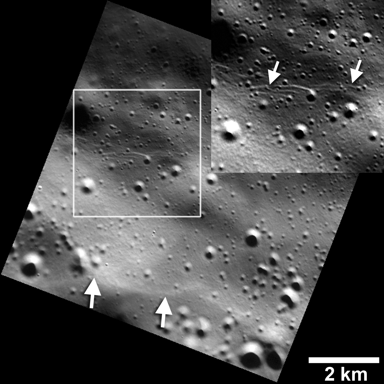
For example, images that were recently obtained by the NASA spacecraft revealed previously undetected landforms – small fault scarps – that appear to be geologically young. The presence of these features have led scientists to conclude that Mercury is still contracting over time, which means that – like Earth – it is tectonically active.
In geology, fault scarps refer to small step-like formations in the surface of a planet, where one side of a fault has moved vertically relative to the other. Previously, scientists believed that Mercury was tectonically dead, and that all major geological activity had taken place in the planet’s early history.
Images showing small fault scarps and trough (lower and upper white arrows) found on Mercury;s surface. Credits: NASA/JHUAPL/Carnegie Institution of Washington/Smithsonian Institution
This was evidenced by features spotted by the MESSENGER and Mariner 10 probes, both of which found evidence of large wrinkle ridges and fault scarps on the surface. The features were reasoned to be the result of Mercury contacting as it cooled early in its history (i.e. billion of years ago).
This action caused the planet’s crust to break, forming cliffs up to a kilometer and a half (about 1 mile) in height and hundreds of kilometers long. However, as the MESSENGER team noted, these small scarps were considerably younger, dating to about 50 million years of age.
They concluded that the scarps would have to be this young in order to survive bombardment by comets and meteoroids, a common occurrence on Mercury. They also noted their resemblance to similar features on the Moon, which also has young scarps that are the result of recent contraction.
“The young age of the small scarps means that Mercury joins Earth as a tectonically active planet, with new faults likely forming today as Mercury’s interior continues to cool and the planet contracts.”
The findings were made during the last 18 months of the MESSENGER mission, during which time the probe lowered its altitude to get higher-resolution images of the planet’s surface. The findings are also consistent with recent findings about Mercury’s global magnetic field, which appears to be powered by the planet’s slowly-cooling outer core.
As Jim Green, NASA’s Planetary Science Director, said of the discovery:
“This is why we explore. For years, scientists believed that Mercury’s tectonic activity was in the distant past. It’s exciting to consider that this small planet – not much larger than Earth’s moon – is active even today.”
All told, these findings have let scientists know that the planet is still alive, in the geological sense. It also means that that there is likely such as thing as Mercury-quakes, something which NASA is sure to follow up on if and when a lander mission (equipped with seismology instruments) is dispatched to the surface of the planet.
Canadians don’t have much to be proud of, but we can regale you with our ability to withstand freezing cold temperatures. Now, I live on the West Coast, so I’m soft and weak, rarely experiencing temperatures below freezing.
But for some of my Canadian brethren, temperatures can dip down to levels your mind and body can scarcely comprehend. For example, I have a friend who lives in Winnipeg, Manitoba. For a day last winter, the temperatures there dipped down -31C, but with the windchill, it felt like -50C. On that same day, it was a balmy -29C on Mars. On Mars!
But for scientists, and the Universe, it can get much much colder. So cold, in fact, that they use a completely different temperature scale – Kelvin – to measure how far away things are from the coldest possible temperature: Absolute Zero.
Nowhere close to absolute zero. Credit: Osccarr (CC BY 2.0)
On the Celsius scale, Absolute Zero is -273.15 degrees. And in Fahrenheit, it’s -459.67 degrees. In the Kelvin scale, however, it’s very simple. Absolute Zero is 0 kelvin.
At this point, a science explainer is going to stumble into a minefield of incorrect usage. It’s not 0 degrees kelvin, you don’t say the degrees part, just the kelvin part. Just kelvin.
This is because when you measure something from an arbitrary point, like the direction you just turned, you’ve changed course 15-degrees. But if you’re measuring from an absolute point, like the lowest physical temperature defined by nature, you drop the degrees because it’s an absolute. An Absolute Zero.
Of course, I’ve probably gotten that wrong too. This stuff is hard.
Anyway, back to Absolute Zero.
Still not cold enough. Credit: Lori Cuthbert (CC BY 2.0)
Absolute Zero is the coldest possible temperature that can theoretically be reached. At this point, no heat energy can be extracted from a system, no work can be done. It’s dead Jim.
But it’s completely theoretical. It’s practically impossible to cool something down to Absolute Zero. In order to cool something down, you need to do work to extract heat from it. The colder you get, the more work you need to do. In order to get to Absolute Zero, you’d need to put in an infinite amount of work. And that’s ridiculous.
As you probably learned in physics or chemistry class, the temperature of a gas translates to the motion of the particles in the gas. As you cool a gas down, by extracting heat from it, the particles slow down.
You would think, then, that by cooling something down to Absolute Zero, all particle motion in that something would stop. But that’s not true.
From a quantum mechanics point of view, you can never know the position and momentum of particles at the same time. If the particles stopped, you’d know their momentum (zero) and their position… right there. The Universe and its laws of physics just can’t allow that to happen. Thank Heisenberg’s Uncertainty Principle.
Therefore, there’s always a little motion, even if you could get to Absolute Zero, which you can’t. But you can’t extract any more heat from it.
The physicist Robert Boyle was one of the first to consider the possibility that there was a lowest possible temperature, which he called the primum frigidum. In 1702, Guillaume Amontons created a thermometer that he calculated would bottom out at -240 C. Pretty close, actually.
But it was Lord Kelvin, who created this absolute scale in 1848, starting at -273 C, or 0 kelvin.
A photograph of Lord Kelvin.
By this measurement, even with its windchill, Winnipeg was a balmy 223 kelvin on that wintry day.
The surface of Pluto, on the other hand varies from a low of 33 kelvin to a high of 55 kelvin. That’s -240 C to -218 C.
The average background temperature across the entire Universe is just 2.7 kelvin. You won’t find many places that cold, unless you get out to the vast cosmic voids that separate galaxy clusters.
Over time, the background temperature of the Universe will continue to drop, but it’ll never actually reach Absolute Zero. Even in a Googol years, when the last supermassive black hole has finally evaporated, and there’s no usable heat left in the entire Universe.
In fact, astronomers call this bleak future the “heat death” of the Universe. It’s heat death, as in, the death of all heat. And happiness.
You might be surprised to know that the coldest temperature in the entire Universe is right here on Earth. Well, sometimes, anyway. And assuming the aliens haven’t got better technology than us, which they probably do.
At the time that I’m recording this video, physicists have used lasers to cool down Rubidium-87 gas to just 170 nanokelvin, a tiny fraction above Absolute Zero. In fact, they won a Nobel Prize for their work in discovering Bose-Einstein condensates.
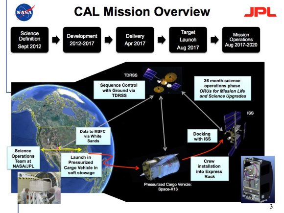
NASA is actually working on a new experiment called the Cold Atom Lab that will send a version of this technology to the International Space Station, where it should be able to cool material down to 100 picokelvin. That’s cold.
The Cold Atom Lab is planned to launch in August 2017. Credit: NASA / JPL
Here are your takeaways. Absolute Zero is the coldest possible temperature than can ever be reached, the point at which no further heat energy can be extracted from a system. Never say degrees kelvin, you’ll cause so much wincing. The Universe can’t match our cold generating abilities… yet. Take that Universe.
I’d love to hear the coldest temperature you’ve ever personally experienced. For me, it was visiting Buffalo in December. That’s not right.
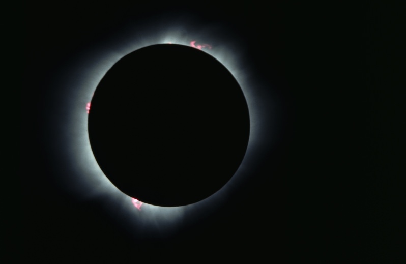
09 March 2016 - Total Solar Eclipse from Palu, Indonesia. Credit and copyright: Justin Ng.
Imagine if you will, that you are a human being living in prehistoric times. You look up at the sky and see the Sun slowly being blocked out, becoming a ominous black sphere that glows around the edges. Could you really be faulted for thinking that this was some sort of supernatural event, or that the end of the world was nigh?
Of course not. Which is why for thousands of years, human beings believed that solar eclipses were just that – a sign of death or a bad omen. But in fact, an eclipse is merely what happens when one stellar object passes in front of another and obscures it. In astronomy, this happens all the time; and between the Sun, the Moon, and the Earth, total eclipses have been witnessed countless times throughout history.
Definition:
The general term for when one body passes in front of another in a solar system is transit. This term accurately describes how, depending on your vantage point, stellar bodies pass in front of each other on a regular basis, thus causing the reflected light from that body to be temporarily obscured.
However, when we are talking about how the Moon can pass between the Earth and the Sun, and how the Earth can pass between the Sun and the Moon, we use the term eclipse. This is also known as a syzygy, an astronomical term derived from ancient Greek (meaning “yoked together”) that describes a straight-line configuration between three celestial bodies.
Total Solar Eclipse:
When the Moon passes between the Sun and the Earth, and the Moon fully occults (blocks) the Sun, it is known as the solar eclipse. The type of solar eclipse – total or partial – depends on the distance of the Moon from the Earth during the event.
During an eclipse of the Sun, only a thin path on the surface of the Earth is actually able to experience a total eclipse – which is called the path of totality. People on either side of that path see a partial eclipse, where the Sun is only partly obscured by the Moon, relative to those who are standing in the center and witnessing the maximum point of eclipse.
A total solar eclipse occurs when the Earth intersects the Moon’s umbra – i.e. the innermost and darkest part of its shadow. These are relatively brief events, generally lasting only a few minutes, and can only be viewed along a relatively narrow track (up to 250 km wide). The region where a partial eclipse can be observed is much larger.
Totality! The view of the last total solar eclipse to cross a U.S. state (Hawaii) back in 1991. Credit and copyright: A. Nartist (shot from Cabo San Lucas, Baja California).
During a solar eclipse, the Moon can sometimes perfectly cover the Sun because its size is nearly the same as the Sun’s when viewed from the Earth. This, of course, is an illusion brought on by the fact that the Moon is much closer to us than the Sun.
And since it is closer, it can block the light from the Sun and cast a shadow on the surface of the Earth. If you’re standing within that shadow, the Sun and the Moon appear to line up perfectly, so that the Moon is completely darkened.
After a solar eclipse reaches totality, the Moon will continue to move past the Sun, obscuring smaller and smaller portions of it and allowing more and more light to pass.
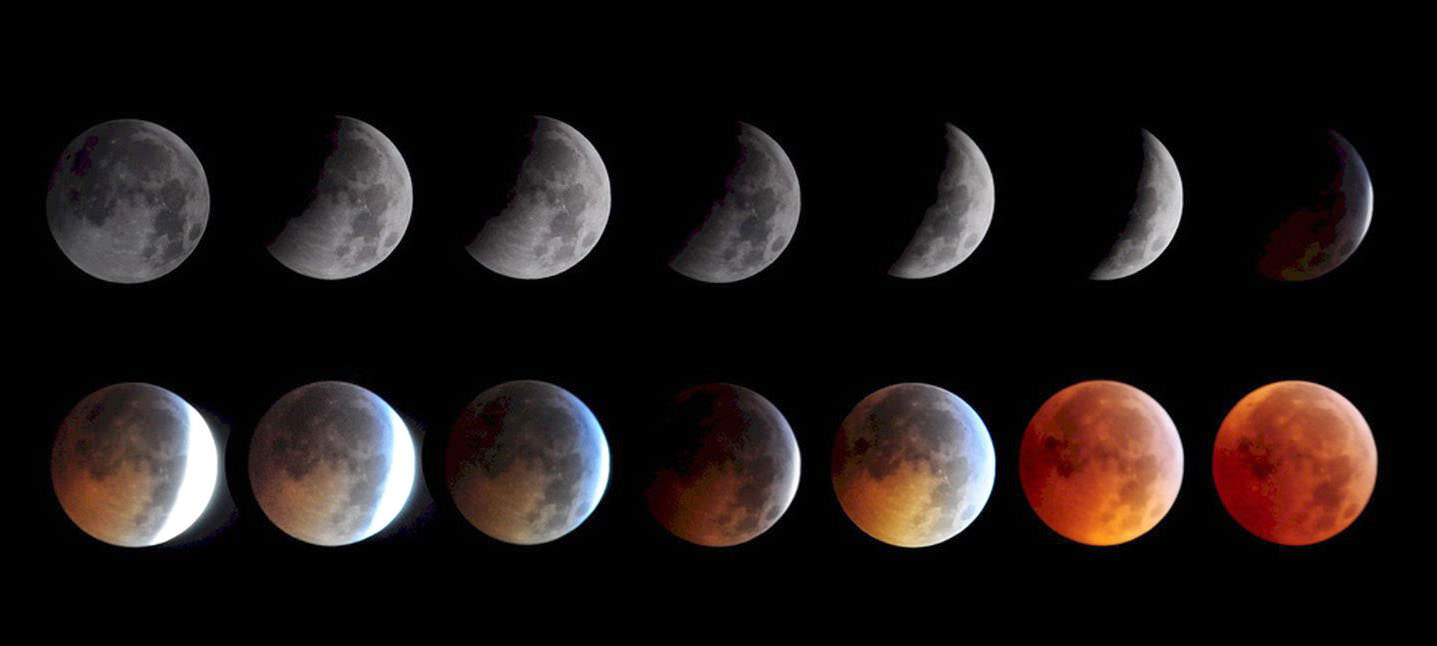
Total Lunar Eclipse:
A total eclipse of the Moon is a different story. In this situation, the entire Moon passes into the Earth’s shadow, darkening it fully. A partial lunar eclipse occurs when the shadow of the Earth doesn’t fully cover the Moon, so only part of the Moon is darkened.
The phases of a total lunar eclipse. Saturday’s eclipse will see the briefest totality in a century. Credit: Keith Burns / NASA
Unlike a solar eclipse, a lunar eclipse can be observed from nearly anywhere in an entire hemisphere. In other words, observers all across planet Earth can see this darkening and it appears the same to all. For this reason, total lunar eclipses are much more common and easier to observe from a given location. A lunar eclipse also lasts longer, taking several hours to complete, with totality itself usually averaging anywhere from about 30 minutes to over an hour.
There are three types of lunar eclipses. There’s a penumbral eclipse, when the Moon crosses only the Earth’s penumbra (the region in which only a portion of light is obscured); followed by a partial, when the Moon crosses partially into the Earth’s umbra (where the light is completely blocked).
Last, there is a total eclipse, when the Moon crosses entirely into the Earth’s umbra. A total lunar eclipse involves the Moon passing through all three phases, then gradually passing out of the Earth’s shadow and becoming bright again. Even during a total lunar eclipse, however, the Moon is not completely dark.
Sunlight is still refracted through the Earth’s atmosphere and enters the umbra to provide faint illumination. Similar to what happens during a sunset, the atmosphere scatters shorter wavelength light, causing it to take on a red hue. This is where the phrase ‘Blood Moon‘ comes from.
Since the Moon orbits the Earth, you would expect to see an eclipse of the Sun and the Moon once a lunar month. However, this does not happen simply because the Moon’s orbit isn’t lined up with the Sun. In fact, the Moon’s orbit is tilted by a few degrees – 1.543º between the angle of the ecliptic and the lunar equator, to be exact.
This means that three objects only have the opportunity to line up and cause an eclipse a few times a year. It’s possible for a total of 7 solar and lunar eclipses every year, but that only happens a few times every century.
Other Types of Eclipses:
The term eclipse is most often used to describe a conjunction between the Earth, Sun and Moon. However, it can also refer to such events beyond the Earth–Moon system. For example, a planet moving into the shadow of one of its moons, a moon passing into the shadow of its host planet, or a moon passing into the shadow of another moon.
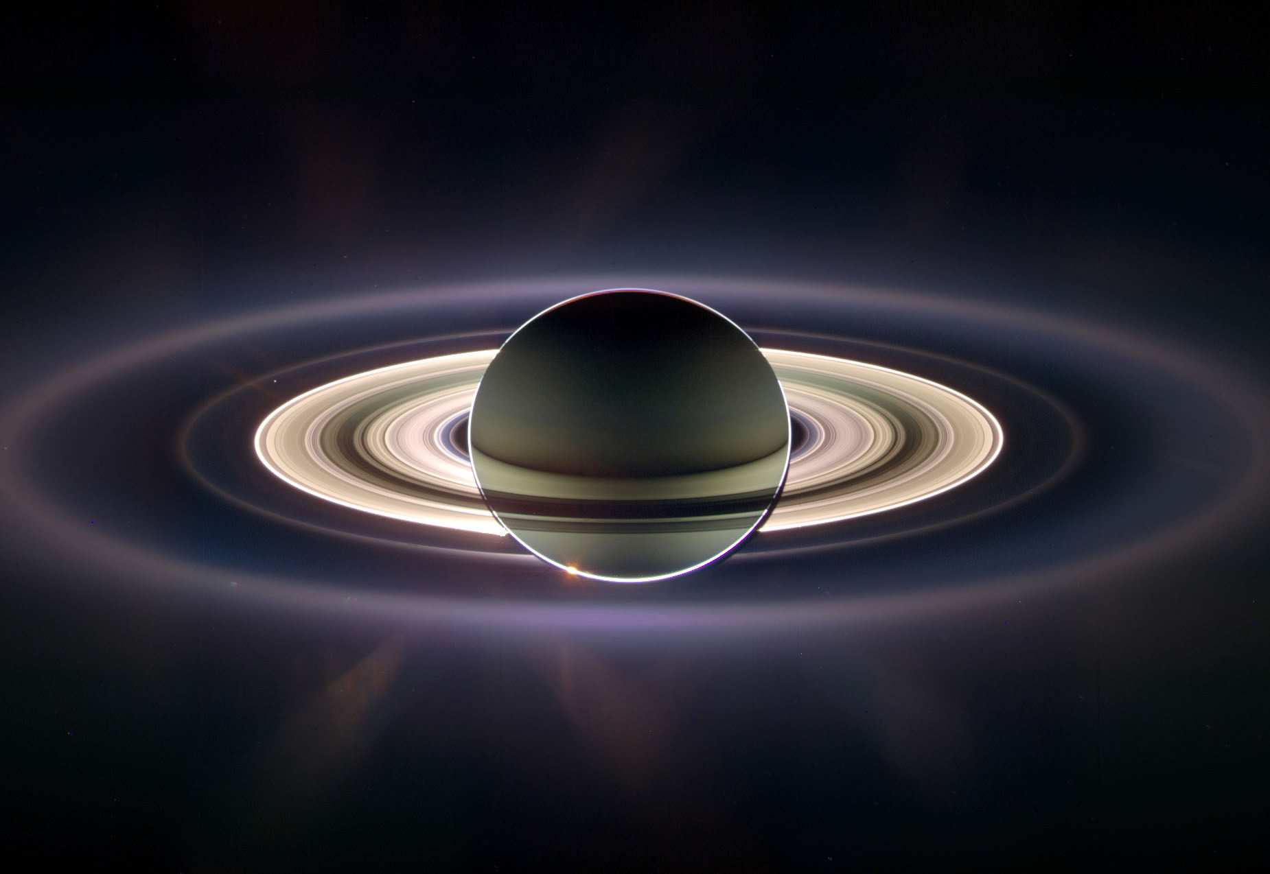
Mosaic of Saturn seen in eclipse in September 2006. Earth is the bright dot just inside the F ring at upper left. (CICLOPS/NASA/JPL-Caltech/SSI)
For instance, during the Apollo 12 mission in 1969, the crew was able to observe the Sun being eclipsed by the Earth. In 2006, during its mission to study Saturn, the Cassini spacecraft was able to capture the image above, which shows the gas giant transiting between the probe and the Sun.
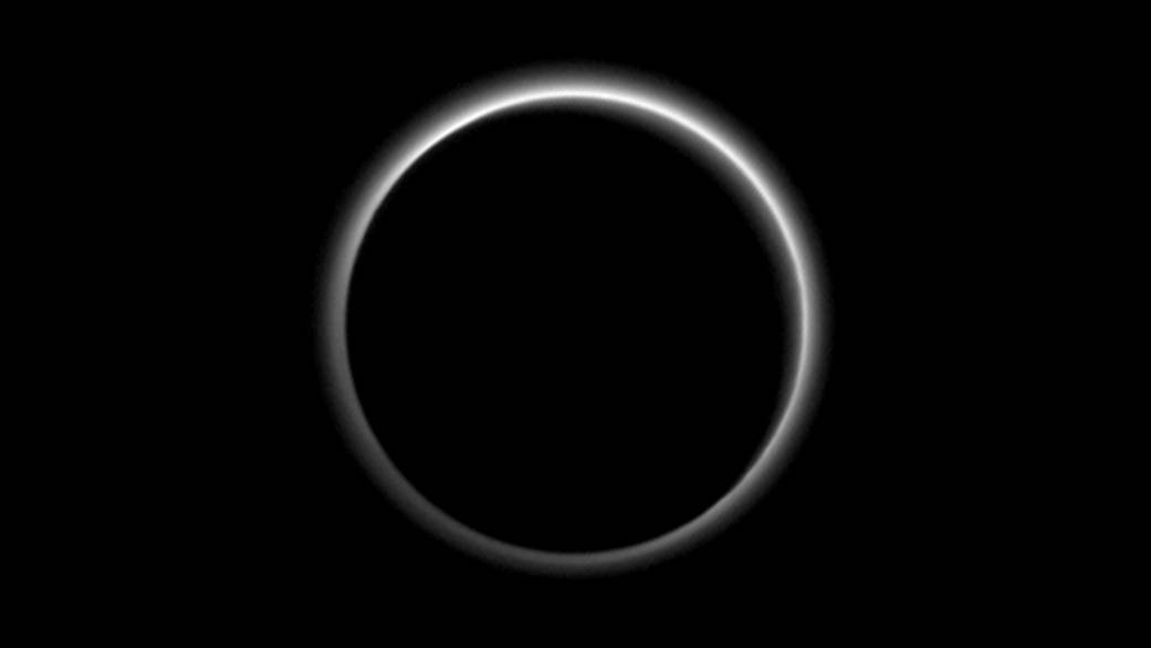
In July of 2015, when the New Horizons mission passed through the shadow of Pluto, it was able to capture a stunning image of the dwarf planet eclipsing the Sun. The image was taken at a distance of about 2 million km (1.25 million miles), which provided the necessary vantage point to see the disc of the Sun become fully obscured.
On top of that, many other bodies in the Solar System can experience eclipses as well. These include the four gas giants, all of which have major moons that periodically transit between the planet and either Earth-based or space-based observatories.
The most impressive and common of these involve Jupiter and its four largest moons (Io, Europa, Ganymede and Callisto). Given the size and low axial tilt of these moons, they often experience eclipses with Jupiter as a result of transits, relative to our instruments.
An enviable view, of the most distant eclipse seen yet, as New Horizons flies through the shadow of Pluto. Credit: NASA/JPL.
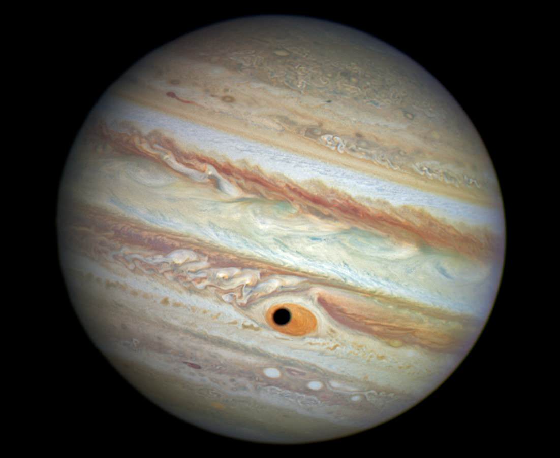
A well-known example occurred in April of 2014, when the Hubble Space Telescope caught an image of Ganymede passing in front at of Jupiter. At the time the image was taken, Ganymede was casting its shadow within Jupiter’s Great Red Spot, which lent the planet a cyclops-like appearance (see below).
The other three gas giants are known to experiences eclipses as well. However, these only occur at certain periods the planet’s orbit of the Sun, due to their higher inclination between the orbits of their moons and the orbital plane of the planets. For instance, Saturn’s largest moon Titan has been known to only occult the ringed gas giant once about every 15 years.
Pluto has also been known to experience eclipses with is largest moon (and co-orbiting body) Charon. However, in all of these cases, the eclipses are never total, as they do not have the size to obscure the much larger gas giant. Instead, the passage of the moons in front of the larger celestial bodies either cast small shadows on the cloud tops of the gas giants, or lead to an annular eclipse at most.
Similarly, on Mars, only partial solar eclipses are ever possible. This is because Phobos or Deimos are not large enough (or distant enough in their orbits) to cover the Sun’s disc, as seen from the surface of the planet. Phobos and Deimos have also been known to experience lunar eclipses as they slip into the shadow of Mars.
Jupiter’s Great Red Spot and Ganymede’s Shadow. Image Credit: NASA/ESA/A. Simon (Goddard Space Flight Center)
Martian eclipses have been photographed numerous times from both the surface and from orbit. For example, in 2010, the Spirit rover captured images of a Martian lunar eclipse as Phobos, the larger of the two martian moons, was photographed while slipping into the shadow of Mars.
Also, between Nov. 4 and Nov. 5, 2010, the Opportunity rover captured several images (later turned into movies) of a Martian sunset. In the course of imaging the Sun for a total of 17 minutes, Opportunity captured stills of the Sun experiencing a solar eclipse. And on September 13th, 2012 – during the 37th day of its mission (Sol 27) – the Curiosity rover captured an image of Phobos transiting the Sun.
As far as astronomical events go, total eclipses (Lunar and Solar) are not uncommon occurrences. If you ever want to witness a one, all you need to do is keep track of when one will be visible from your part of the world. Some good resources for this are NASA’s Eclipse Website and timeanddate.com.
Or, if you’re the really adventurous type, you can find out where on Earth the next path of totality is going to be, and then book a vacation to go there. Get to the right spot at the right time, and you should be getting the view of a lifetime!
We have written many articles about the eclipse for Universe Today. Here’s a list of articles about specific times when a total Lunar Eclipse took place, and here’s a list of Solar Eclipse articles. And be sure to check out this article and video of an Annular Eclipse.
Artist's impression of a water vapor plume on Europa. Credit: NASA/ESA/K. Retherford/SWRI
Last week, on Tuesday, September 20th, NASA announced that they had made some interesting findings about Jupiter’s icy moon Europa. These were based on images taken by the Hubble Space Telescope, the details of which would be released on the following week. Needless to say, since then, the scientific community and general public have been waiting with baited breath.
Earlier today (September 26th) NASA put an end to the waiting and announced the Hubble findings during a NASA Live conference. According to the NASA panel, which was made up of members of the research team, this latest Europa-observing mission revealed evidence of plumes of saline water emanating from Europa’s surface. If true, this would mean that the moon’s subsurface ocean would be more accessible than previously thought.
Using Hubble’s Space Telescope Imaging Spectrograph (STIS) instrument, the team conducted observations of Jupiter and Europa in the ultra-violet spectrum over the course of 15 months. During that time, Europa passed in front of Jupiter (occulted the gas giant) on 10 separate occasions.
And on three of these occasions, the team saw what appeared to be plumes of water erupting from the surface. These plumes were estimated to be reaching up to 200 km (125 miles) from the southern region of Europa before (presumably) raining back onto the surface, depositing water ice and material from the interior.
The purpose of the observation was to examine Europa’s possible extended atmosphere (aka. exosphere). The method the team employed was similar to the one used to detect atmospheres around extra-solar planets. As William Sparks of the Space Telescope Science Institute (STScI) in Baltimore (and the team leader), explained in a NASA press release:
“The atmosphere of an extrasolar planet blocks some of the starlight that is behind it. If there is a thin atmosphere around Europa, it has the potential to block some of the light of Jupiter, and we could see it as a silhouette. And so we were looking for absorption features around the limb of Europa as it transited the smooth face of Jupiter.”
When they looked at Europa using this same technique, they noted that small patches on the surface were dark, indicating the absorption of UV light. This corresponded to previous work done by Lorenz Roth (of the Southwest Research Institute) and his team of researchers in 2012. At this time, they detected evidence of water vapor coming from Europa’s southern polar region.
Europa transit illustration. Europa orbits Jupiter every 3 and a half days, and on every orbit it passes in front of Jupiter, raising the possibility of plumes being seen as silhouettes absorbing the background light of Jupiter. Credits: A. Field (STScI)
As they indicated in a paper detailing their results – titled “Transient Water Vapor at Europa’s South Pole” – Roth’s team also relied on UV observations made using the Hubble telescope. Noting a statistically coincident amount of hydrogen and oxygen emissions, they concluded that this was the result of ejected water vapor being broken apart by Jupiter’s radiation (a process known as radiolysis).
Though their methods differed, Sparks and his research team also found evidence of these apparent water plumes, and in the same place no less. Based on the latest information from STIS, most of the apparent plumes are located in the moon’s southern polar region while another appears to be located in the equatorial region.
“When we calculate in a completely different way the amount of material that would be needed to create these absorption features, it’s pretty similar to what Roth and his team found,” Sparks said. “The estimates for the mass are similar, the estimates for the height of the plumes are similar. The latitude of two of the plume candidates we see corresponds to their earlier work.”
Another interesting conclusion to come from this and the 2012 study is the likelihood that these water plumes are intermittent. Basically, Europa is tidally-locked world, which means the same side is always being presented to us when it transits Jupiter. This occus once every 3.5 days, thus giving astronomers and planetary scientists plenty of viewing opportunities.
This composite image shows suspected plumes of water vapor erupting at the 7 o’clock position off the limb of Jupiter’s moon Europa. The Hubble data were taken on January 26, 2014. Credit: Credits: NASA/ESA/W. Sparks (STScI)/USGS Astrogeology Science Center
But the fact that plumes have been observed at some points and not others would seem to indicate that they are periodic. In addition, Roth’s team attempted to spot one of the plume’s observed by Sparks and his colleagues a week after they reported it. However, they were unable to locate this supposed water source. As such, it would appear that the plumes, if they do exist, are short-lived.
These findings are immensely significant for two reasons. On the one hand, they are further evidence that a warm-water, saline ocean exists beneath Europa’s icy surface. On the other, they indicate that any future mission to Europa would be able to access this salt-water ocean with greater ease.
Ever since the Galileo spacecraft conducted a flyby of the Jovian moon, scientists have believed that an interior ocean is lying beneath Europa’s icy surface – one that has between two and three times as much water as all of Earth’s oceans combined. However, estimates of the ice’s thickness range from it being between 10 to 30 km (6–19 mi) thick – with a ductile “warm ice” layer that increases its total thickness to as much as 100 km (60 mi).
Knowing the water periodically reaches the surface through fissures in the ice would mean that any future mission (which would likely include a submarine) would not have to drill so deep. And considering that Europa’s interior ocean is considered to be one of our best bets for finding extra-terrestrial life, knowing that the ocean is accessible is certainly exciting news.
A comparison of 2014 transit and 2012 Europa aurora observations. Credits: NASA, ESA, W. Sparks (left image) L. Roth (right image)
And the news is certainly causing its fair share of excitement for the people who are currently developing NASA’s proposed Mission to Europa, which is scheduled to launch sometime in the 2020s. As Dr. Cynthia B. Phillips, a Staff Scientist and the Science Communications Lead for the Europa Project, told Universe Today via email:
“This new discovery, using Hubble Space Telescope data, is an intriguing data point that helps lend support to the idea that there are active plumes on Europa today. While not an absolute confirmation, the new Sparks et al. result, in combination with previous observations by Roth et al. (also using HST but with a different technique), is consistent with the presence of intermittent plumes ejecting water vapor from the Southern Hemisphere of Europa. Such observations are difficult to perform from Earth, however, even with Hubble, and thus these results remain inconclusive.
“Confirming the presence or absence of plumes on Europa, as well as investigating many other mysteries of this icy ocean world, will require a dedicated spacecraft in the Jupiter system. NASA currently plans to send a multiple-flyby spacecraft to Europa, which would make many close passes by Europa in the next decade. The spacecraft’s powerful suite of scientific instruments will be able to study Europa’s surface and subsurface in unprecedented detail, and if plumes do exist, it will be able to observe them directly and even potentially measure their composition. Until the Europa spacecraft is in place, however, Earth-based observations such as the new Hubble Space Telescope results will remain our best technique to observe Jupiter’s mysterious moon.”
Naturally, Sparks was clear that this latest information was not entirely conclusive. While he believes that the results were statistically significant, and that there were no indications of artifacts in the data, he also emphasized that observations conducted in the UV wavelength are tricky. Therefore, more evidence is needed before anything can be said definitively.
In the future, it is hoped that future observation will help to confirm the existence of water plumes, and how these could have helped create Europa’s “chaos terrain”. Future missions, like NASA’s James Webb Space Telescope (scheduled to launch in 2018) could help confirm plume activity by observing the moon in infrared wavelengths.
As Paul Hertz, the director of the Astrophysics Division at NASA Headquarters in Washington, said:
“Hubble’s unique capabilities enabled it to capture these plumes, once again demonstrating Hubble’s ability to make observations it was never designed to make. This observation opens up a world of possibilities, and we look forward to future missions — such as the James Webb Space Telescope — to follow up on this exciting discovery.”
Other team members include Britney Schmidt, an assistant professor at the School of Earth and Atmospheric Sciences at Georgia Institute of Technology in Atlanta; and Jennifer Wiseman, senior Hubble project scientist at NASA’s Goddard Space Flight Center in Greenbelt, Maryland. Their work will be published in the Sept. 29 issue of the Astrophysical Journal.
And be sure to enjoy this video by NASA about this exciting find:
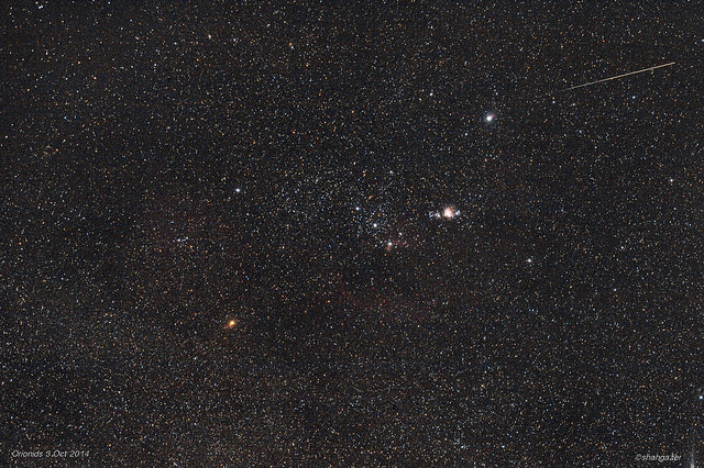
A 2014 Orionid meteor. Image credit and copright: Sharin Ahmad (@Shahgazer).
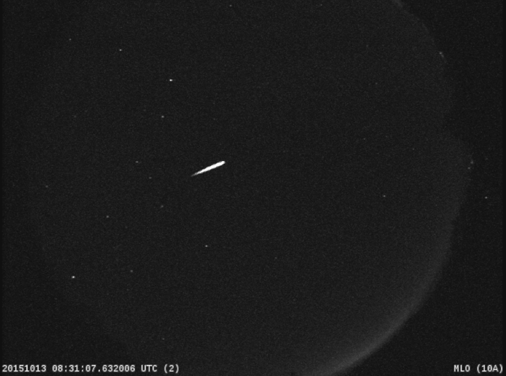
The month of October is upon us this coming weekend, and with it, one of the better annual meteor showers is once again active: the Orionids.
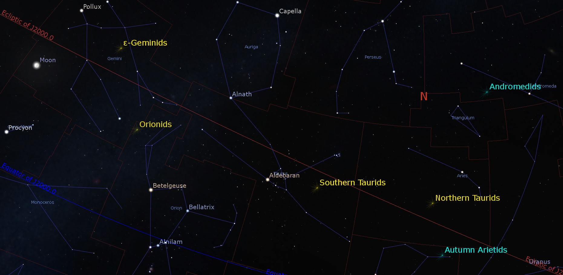
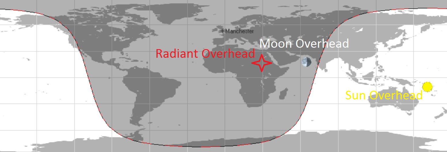
In 2016, the Orionid meteors are expected to peak on October 22nd at 2:00 UT (10:00 PM U.S. Eastern Time on October 21st) , favoring Europe and Africa in the early morning hours. The shower is active for a one month period from October 2nd to November 2nd, and can vary with a Zenithal Hourly Rate (ZHR) of 10-70 meteors per hour. This year, the Orionids are expected to produce a maximum ideal ZHR of 15-25 meteors per hour. The radiant of the Orionids is located near right ascension 6 hours 24 minutes, declination 15 degrees north at the time of the peak. The radiant is in the constellation of Orion very near its juncture with Gemini and Taurus.
A gallery of Fall meteor shower radiants, including the October Orionids. Image credit: Stellarium
The Moon is at a 55% illuminated, waning gibbous phase at the peak of the Orionids, making 2016 an unfavorable year for this shower, though that shouldn’t stop you from trying. It’s true that the Moon is only 19 degrees east of the radiant in the adjacent constellation Gemini at its peak on the key morning of October 22, though it’ll move farther on through the last week of October.
In previous recent years, the Orionids produced a Zenithal Hourly Rate (ZHR) of 20 (2014) and a ZHR of 30 (2013).
The Orionid meteors strike the Earth at a moderately fast velocity of 66 km/s, and the shower tends to produce a relatively high ratio of fireballs with an r value of = 2.5. The source of the Orionids is none other than renowned comet 1/P Halley. Halley last paid the inner solar system a visit in early 1986, and will once again reach perihelion on July 28, 2061. Let’s see, by then I’ll be…
The orientation of the Earth’s shadow vs the zenith positions of the Sun, Moon and the radiant of the Orionid meteors at the expected during the peak of the shower on October 22nd. Image adapted from Orbitron.
Unlike most meteor showers, the Orionids display a very unpredictable maximum – many sources decline to put a precise date on the shower’s expected maximum at all. On some years, the Orionids barely top 10 per hour at their maximum, while on others they display a broad but defined peak. One 1982 study out of Czechoslovakia suggested a twin peak for this shower after looking at activity from 1944 to 1950. All good reasons to be vigilant for Orionids throughout the coming month of October.
And check out this brilliant meteor that lit up the skies over the southern UK this past weekend:
‘Tis the season for cometary dust particles to light up the night sky. Trace the path of a suspect meteor to the club of Orion, and you’ve likely sighted an Orionid meteor. But other showers showers are active in October, including:
The Draconids: Peaking around October 8th, these are debris shed by Comet 21P Giacobini-Zinner. The Draconids are prone to great outbursts, such as the 2011 and 2012 meteor storm, but are expected to yield a paltry ZHR of 10 in 2016.
The Taurids: Late October into early November is Taurid fireball season, peaking with a ZHR of 5 around October 10th (the Southern Taurids) and November 12th (the Northern Taurids).
The Camelopardalids: Another wildcard shower prone to periodic outbursts. 2016 is expected to be an off year for this shower, with a ZHR of 10 topping out on October 5.
And farther afield, we’ve got the Leonids (November 17th) the Geminids (December 14th) and the Ursids (December 22nd) to close out 2016.
A 2015 Orionid captured by a NASA All-Sky camera atop Mt. Lemmon, Arizona. Image credit: NASA.
Observing a meteor shower like the Orionids is as simple as finding a dark site with a clear horizon, laying back and watching via good old Mark-1 eyeball. Blocking that gibbous Moon behind a building or hill will also increase your chances of catching an Orionid. Expect rates to pick up toward dawn, as the Earth turns forward and plows headlong into the meteor stream.
You can make a count of what you see and report it to the International Meteor Organization which keeps regular tabs of meteor activity.
Photographing Orionids this year might be problematic, owing to the proximity of the bright Moon, though not impossible. Again, aiming at a wide quadrant of the sky opposite to the Moon might just nab a bright Orionid meteor in profile. We like to just set our camera’s intervalometer to take a sequence of 30” exposures of the sky, and let it do the work while we’re observing visually. Nearly every meteor we’ve caught photographically turned up in later review, a testament to the limits of visual observing.
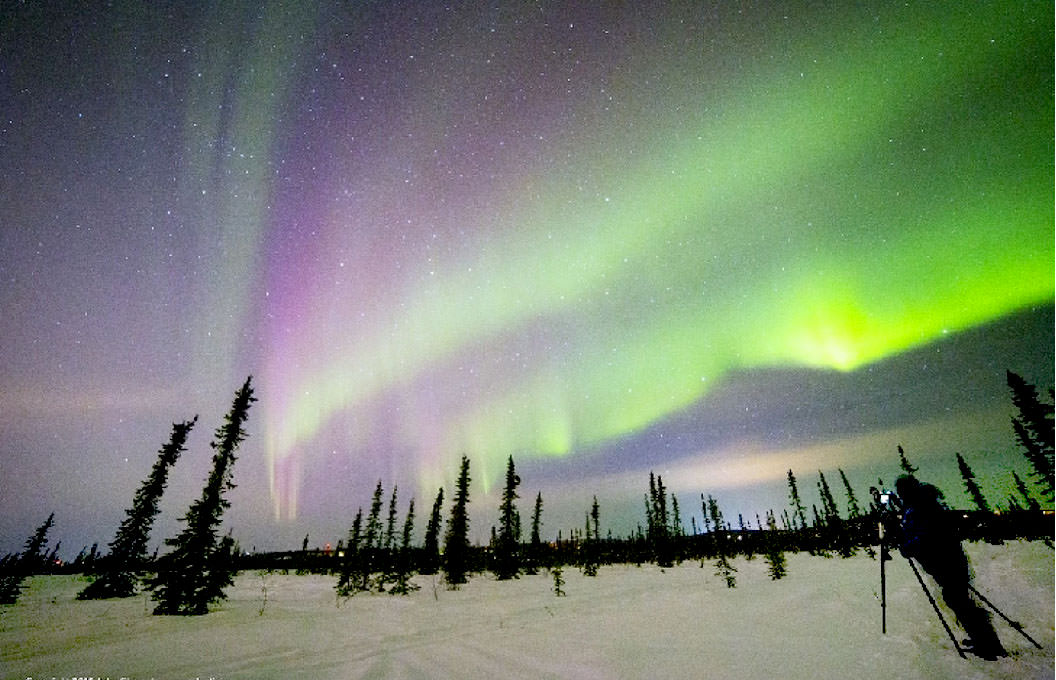
Aurora borealis in Fairbanks, AK. on Monday night March 16. Credit: John Chumack
The Northern Lights have fascinated human beings for millennia. In fact, their existence has informed the mythology of many cultures, including the Inuit, Northern Cree, and ancient Norse. They were also a source of intense fascination for the ancient Greeks and Romans, and were seen as a sign from God by medieval Europeans.
Thanks to the birth of modern astronomy, we now know what causes both the Aurora Borealis and its southern sibling – Aurora Australis. Nevertheless, they remain the subject of intense fascination, scientific research, and are a major tourist draw. For those who live north of 60° latitude, this fantastic light show is also a regular occurrence.
Causes:
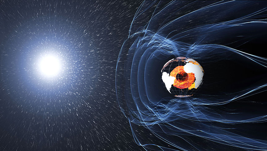
Aurora Borealis (and Australis) is caused by interactions between energetic particles from the Sun and the Earth’s magnetic field. The invisible field lines of Earth’s magnetoshere travel from the Earth’s northern magnetic pole to its southern magnetic pole. When charged particles reach the magnetic field, they are deflected, creating a “bow shock” (so-named because of its apparent shape) around Earth.
However, Earth’s magnetic field is weaker at the poles, and some particles are therefore able to enter the Earth’s atmosphere and collide with gas particles in these regions. These collisions emit light that we perceive as wavy and dancing, and are generally a pale, yellowish-green in color.
The variations in color are due to the type of gas particles that are colliding. The common yellowish-green is produced by oxygen molecules located about 100 km (60 miles) above the Earth, whereas high-altitude oxygen – at heights of up to 320 km (200 miles) – produce all-red auroras. Meanwhile, interactions between charged particles and nitrogen will produces blue or purplish-red auroras.
Variability:
The visibility of the northern (and southern) lights depends on a lot of factors, much like any other type of meteorological activity. Though they are generally visible in the far northern and southern regions of the globe, there have been instances in the past where the lights were visible as close to the equator as Mexico.
In places like Alaska, Norther Canada, Norway and Siberia, the northern lights are often seen every night of the week in the winter. Though they occur year-round, they are only visible when it is rather dark out. Hence why they are more discernible during the months where the nights are longer.
The magnetic field and electric currents in and around Earth generate complex forces, and also lead to the phenomena known as aurorae. Credit: ESA/ATG medialab
Because they depend on the solar wind, auroras are more plentiful during peak periods of activity in the Solar Cycle. This cycle takes places every 11 years, and is marked by the increase and decrease of sunspots on the sun’s surface. The greatest number of sunspots in any given solar cycle is designated as a “Solar Maximum“, whereas the lowest number is a “Solar Minimum.”
A Solar Maximum also accords with bright regions appearing in the Sun’s corona, which are rooted in the lower sunspots. Scientists track these active regions since they are often the origin of eruptions on the Sun, such as solar flares or coronal mass ejections.
The most recent solar minimum occurred in 2008. As of January 2010, the Sun’s surface began to increase in activity, which began with the release of a lower-intensity M-class flare. The Sun continued to get more active, culminating in a Solar Maximum by the summer of 2013.
Locations for Viewing:
The ideal places to view the Northern Lights are naturally located in geographical regions north of 60° latitude. These include northern Canada, Greenland, Iceland, Scandinavia, Alaska, and Northern Russia. Many organizations maintain websites dedicated to tracking optimal viewing conditions.
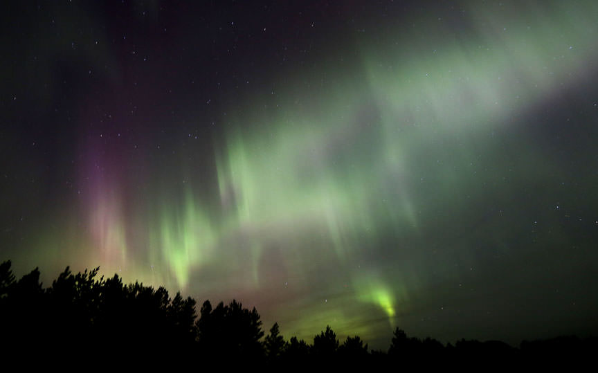
An image captured of the northern lights, which appear pale purple and red, though the primary color visible to the eye was green. Credit: Bob Kin
For instance, the Geophysical Institute of the University of Alaska Fairbanks maintains the Aurora Forecast. This site is regularly updated to let residents know when auroral activity is high, and how far south it will extend. Typically, residents who live in central or northern Alaska (from Fairbanks to Barrow) have a better chance than those living in the south (Anchorage to Juneau).
In Northern Canada, auroras are often spotted from the Yukon, the Northwest Territories, Nunavut, and Northern Quebec. However, they are sometimes seen from locations like Dawson Creek, BC; Fort McMurry, Alberta; northern Saskatchewan and the town of Moose Factory by James Bay, Ontario. For information, check out Canadian Geographic Magazine’s “Northern Lights Across Canada“.
The National Oceanic and Atmospheric Agency also provides 30 minute forecasts on auroras through their Space Weather Prediction Center. And then there’s Aurora Alert, an Android App that allows you to get regular updates on when and where an aurora will be visible in your region.
Understanding the scientific cause of auroras has not made them any less awe-inspiring or wondrous. Every year, countless people venture to locations where they can be seen. And for those serving aboard the ISS, they got the best seat in the house!
Speaking of which, be sure to check out this stunning NASA video which shows the Northern Lights being viewed from the ISS:
For more information, visit the THEMIS website – a NASA mission that is currently studying space weather in great detail. The Space Weather Center has information on the solar wind and how it causes aurorae.
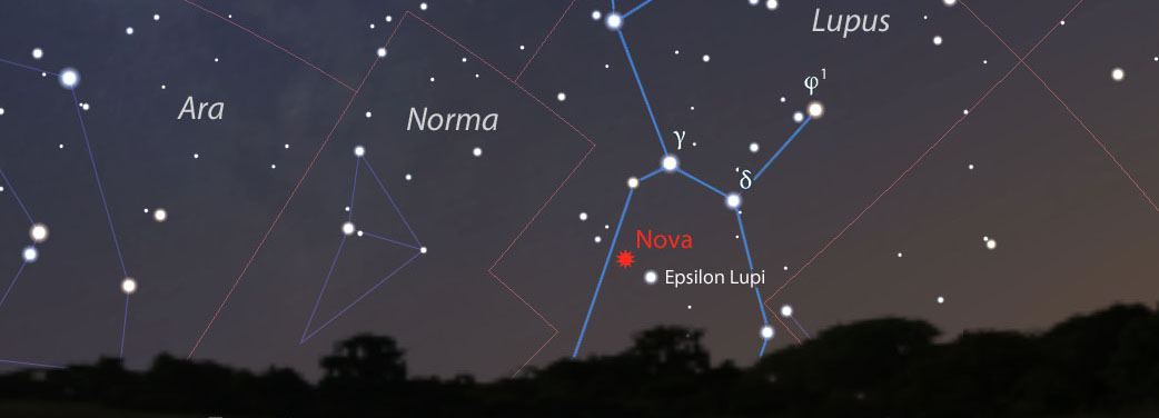
The possible nova in Lupus photographed on Sunday, Sept. 25 from Australia. The star is now bright enough to see in binoculars for observers in the far southern U.S. and points south. Credit: Joseph Brimacombe
On September 20, a particular spot in the constellation Lupus the Wolf was blank of any stars brighter than 17.5 magnitude. Four nights later, as if by some magic trick, a star bright enough to be seen in binoculars popped into view. While we await official confirmation, the star’s spectrum, its tattle-tale rainbow of light, indicates it’s a nova, a sun in the throes of a thermonuclear explosion.
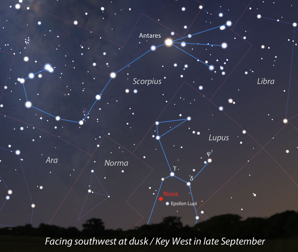
The nova was discovered on Sept. 23 near the 3rd magnitude star Epsilon Lupi. It rose from fainter than magnitude +17.5 to its current magnitude +6.8 in just four nights … and it’s still rising. It’s visible low in the southwestern sky in late evening twilight low northern latitudes, the tropics and southern hemisphere. This map shows the sky facing southwest about an hour after sunset from Key West, Florida, latitude 24.5 degrees north. Source: Stellarium
The nova, dubbed ASASSN-16kt for now, was discovered during the ongoing All Sky Automated Survey for SuperNovae (ASAS-SN or “Assassin”), using data from the quadruple 14-cm “Cassius” telescope in CTIO, Chile. Krzysztof Stanek and team reported the new star in Astronomical Telegram #9538. By the evening of September 23 local time, the object had risen to magnitude +9.1, and it’s currently +6.8. So let’s see — that’s about an 11-magnitude jump or a 24,000-fold increase in brightness! And it’s still on the rise.
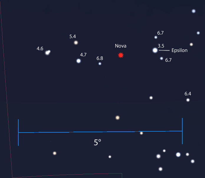
Use this chart with binoculars to help you find the likely nova. The field of view is about 5 degrees with north up. The “new star” lies between a bright triangle of stars to the east and the naked-eye star Epsilon Lupi to the west. Stars are labeled with magnitudes. Chart: Bob King, Source: Stellarium
The star is located at R.A. 15h 29?, –44° 49.7? in the southern constellation Lupus the Wolf. Even at this low declination, the star would clear the southern horizon from places like Chicago and further south, but in late September Lupus is low in the southwestern sky. To see the nova you’ll need a clear horizon in that direction and observe from the far southern U.S. and points south. If you’ve planned a trip to the Caribbean or Hawaii in the coming weeks, your timing couldn’t have been better!
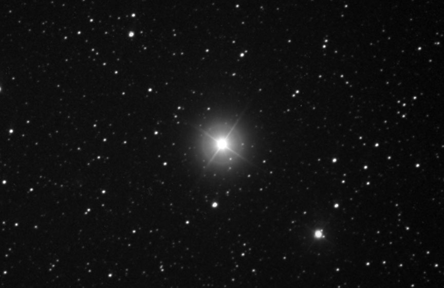
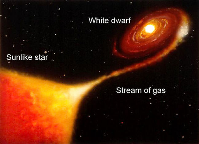
Novae occur in close binary systems where one star is a tiny but extremely compact white dwarf star. The dwarf draws material into a disk around itself, some of which is funneled to the surface and ignites in a nova explosion. Credit: NASA
I’ve drawn the map for Key West, one of southernmost locations on the U.S. mainland, where the nova stands about 7-8° high in late twilight, but you might also see it from southern Texas and the bottom of Arizona if you stand on your tippytoes. Other locales include northern Africa, Finding a good horizon is key. Observers across Central and South America, Africa, India, s. Asia and Australia, where the star is higher up in the western sky at nightfall, are favored.
Nova means “new”, but a nova isn’t a brand new star coming to life but rather an explosion that occurs on the surface of an otherwise faint star no one’s taken notice of – until the blast causes it to brighten 50,000 to 100,000 times.
You can use this AAVSO chart to find the nova and track its changing brightness. Star magnitudes are shown to the tenth with the decimal omitted. Click to enlarge. Credit: AAVSO
A nova occurs in a close binary star system, where a small but extremely dense and massive (for its size) white dwarf siphons hydrogen gas from its closely-orbiting companion. After whirling around in a flattened accretion disk around the dwarf, the material gets funneled down to the star’s 150,000 F° surface where gravity compacts and heats the gas until it detonates in a titanic thermonuclear explosion. Suddenly, a faint star that wasn’t on anyone’s radar vaults a dozen magnitudes to become a standout “new star”.
Novae are relatively rare and almost always found in the plane of the Milky Way, where the stars are most concentrated. The more stars, the greater the chances of finding one in a nova outburst. Roughly a handful a year are discovered, many of those in Scorpius and Sagittarius, in the direction of the galactic bulge.
We’ll keep tabs on this new object and report back with more information and photos as they become available. You can follow the new celebrity as well as print out finder charts on the American Association of Variable Star Observers (AAVSO) website by typing ASASSN-16kt in the info boxes.
I sure wish I wasn’t stuck in Minnesota right now or I’d be staring down the wolf’s new star!
Dramatic wide angle mosaic view of butte with sandstone layers showing cross-bedding in the Murray Buttes region on lower Mount Sharp with distant view to rim of Gale crater, taken by Curiosity rover’s Mastcam high resolution cameras. This photo mosaic was assembled from Mastcam color camera raw images taken on Sol 1454, Sept. 8, 2016 and stitched by Ken Kremer and Marco Di Lorenzo, with added artificial sky. Featured at APOD on 5 Oct 2016. Credit: NASA/JPL/MSSS/Ken Kremer/kenkremer.com/Marco Di Lorenzo
Dramatic wide angle mosaic view of butte with sandstone layers showing cross-bedding in the Murray Buttes region on lower Mount Sharp with distant view to rim of Gale crater, taken by Curiosity rover’s Mastcam high resolution cameras. This photo mosaic was assembled from Mastcam color camera raw images taken on Sol 1454, Sept. 8, 2016 and stitched by Ken Kremer and Marco Di Lorenzo, with added artificial sky. Credit: NASA/JPL/MSSS/Ken Kremer/kenkremer.com/Marco Di Lorenzo
Our beyond magnificent Curiosity rover has just finished her latest Red Planet drilling campaign – at the rock target called “Quela” – into the simply unfathomable alien landscapes she is currently exploring at the “Murray Buttes” region of lower Mount Sharp. And it’s all in a Sols (or Martian Day’s) work for our intrepid Curiosity!
“These images are literally out of this world.. I don’t think I have seen anything like them on Earth!” Jim Green, Planetary Sciences Director at NASA Headquarters, Washington, D.C., explained to Universe Today.
The “Murray Buttes” region is just chock full of the most stunning panoramic vistas that NASA’s Curiosity Mars Science Laboratory rover has come upon to date. Observe and enjoy them in our exclusive new photo mosaics above and below.
“We always try to find some sort of Earth analog but these make exploring another world all worth it!” Green gushed in glee.
They fill the latest incredible chapter in her thus far four year long quest to trek many miles (km) from the Bradbury landing site across the floor of Gale Crater to reach the base region of humongous Mount Sharp.
And these adventures are just a prelude to the even more glorious vistas she’ll investigate from now on – as she climbs higher and higher on an expedition to thoroughly examine the mountains sedimentary layers and unravel billions and billions of years of Mars geologic and climatic history.
Drilling holes into Mars during the Red Planet trek and carefully analyzing the pulverized samples with the rovers pair of miniaturized chemistry laboratories (SAM and CheMin) is the route to the answer of how and why Mars changed from a warmer and wetter planet in the ancient past to the cold, dry and desolate world we see today.
The rock target named “Quela” is located at the base of one of the buttes dubbed “Murray Butte number 12,” according to the latest mission update from Prof. John Bridges, a Curiosity rover science team member from the University of Leicester, England.
It took two tries to get the drilling done due to a technical issue, but all went well in the end and it was well worth the effort at a place never before explored by an emissary from Earth.
“The drill (successful at second attempt) is at Quela.”
The full depth drilling was completed on Sol 1464, Sept. 18, 2016 using the percussion drill at the terminus of the outstretched 7-foot-long (2-meter-long) robotic arm – as confirmed by imaging and further illustrated in our navcam camera photo mosaic.
And that immediately provided valuable insight into climate change on Mars.
“You can see how red and oxidised the tailings are, suggesting changing environmental conditions as we progress through the Mt. Sharp foothills,” Bridges explained in the mission update.
Curiosity bore holes measure approximately 0.63 inch (1.6 centimeters) in diameter and 2.6 inches (6.5 centimeters) deep.
Quela drill hole bored by Curiosity rover on Sol 1464, Sept. 18, 2016 as seen in this collage of Mastcam and MAHLI raw color images taken on Sol 1465. Image Credit: NASA/JPL/MSSS. Collage: Marco Di Lorenzo/Ken Kremer
To give you the context of the Murray Buttes region and the drilling at Quela, the image processing team of Ken Kremer and Marco Di Lorenzo has begun stitching together wide angle mosaic landscape views and up close views of the drilling using raw images from the variety of cameras at Curiosity’s disposal.
The next steps after boring into Quela were to “sieve the new sample, dump the unsieved fraction, and drop some of the sieved sample into CheMin,” says Ken Herkenhoff, Research Geologist at the USGS Astrogeology Science Center and an MSL science team member, in a mission update.
“But first, ChemCam will acquire passive spectra of the Quela drill tailings and use its laser to measure the chemistry of the wall of the new drill hole and of bedrock targets “Camaxilo” and “Okakarara.” Right Mastcam images of these targets are also planned.”
“After sunset, MAHLI will use its LEDs to take images of the drill hole from various angles and of the CheMin inlet to confirm that the sample was successfully delivered. Finally, the APXS will be placed over the drill tailings for an overnight integration.”
The rover had approached the butte from the south side several sols earlier to get in place, plan for the drilling, take imagery to document stratigraphy and make compositional observations with the ChemCam laser instrument.
Curiosity drills into Quela rock target in the Murray Buttes region on Sol 1464, Sept. 18, 2016, in this navcam camera mosaic, stitched from raw images and colorized. Credit: NASA/JPL/Ken Kremer/kenkremer.com/Marco Di Lorenzo
“These are the landforms that dominate the landscape at this point in the traverse – The Murray Buttes,” says Bridges.
Wide angle mosaic view shows spectacular buttes and layered sandstone in the Murray Buttes region on lower Mount Sharp from the Mastcam cameras on NASA’s Curiosity Mars rover. This photo mosaic was assembled from Mastcam color camera raw images taken on Sol 1455, Sept. 9, 2016 and stitched by Marco Di Lorenzo and Ken Kremer, with added artificial sky. Credit: NASA/JPL/MSSS/Ken Kremer/kenkremer.com/Marco Di Lorenzo
What are the Murray Buttes?
“These are formed by a cap of hard aeolian rock that has been partially eroded back, overlying the Murray mudstone.”
The imagery of the Murray Buttes and mesas show them to be eroded remnants of ancient sandstone that originated when winds deposited sand after lower Mount Sharp had formed.
Scanning around the Murray Buttes mosaics one sees finely layered rocks, sloping hillsides, the distant rim of Gale Crater barely visible through the dusty haze, dramatic hillside outcrops with sandstone layers exhibiting cross-bedding.
The presence of “cross-bedding” indicates that the sandstone was deposited by wind as migrating sand dunes, says the team.
Spectacular wide angle mosaic view showing sloping buttes and layered outcrops within the Murray Buttes region on lower Mount Sharp from the Mast Camera (Mastcam) on NASA’s Curiosity Mars rover. This photo mosaic is stitched from Mastcam camera raw images taken on Sol 1454, Sept. 9, 2016 with added artificial sky. Credit: NASA/JPL/MSSS/Ken Kremer/kenkremer.com/Marco Di Lorenzo
Curiosity spent some six weeks or so traversing and exploring the Murray Buttes.
So after collecting all that great drilling data at Quela, the team is ready for even more spectacular new adventures!
“While the Murray Buttes were spectacular and interesting, it’s good to be back on the road again, as there is much more of Mt. Sharp to explore!” concludes Herkenhoff.
And the team is already commanding Curiosity to drive ahead in hot pursuit of the next drill target!
Dramatic hillside view showing sloping buttes and layered outcrops within of the Murray Buttes region on lower Mount Sharp from the Mast Camera (Mastcam) on NASA’s Curiosity Mars rover. This photo mosaic is stitched and cropped from Mastcam camera raw images taken on Sol 1454, Sept. 8, 2016, with added artificial sky. Credit: NASA/JPL/MSSS/Ken Kremer/kenkremer.com/Marco Di Lorenzo
Ascending and diligently exploring the sedimentary lower layers of Mount Sharp, which towers 3.4 miles (5.5 kilometers) into the Martian sky, is the primary destination and goal of the rovers long term scientific expedition on the Red Planet.
Curiosity rover panorama of Mount Sharp captured on June 6, 2014 (Sol 651) during traverse inside Gale Crater. Note rover wheel tracks at left. She will eventually ascend the mountain at the ‘Murray Buttes’ at right later this year. Assembled from Mastcam color camera raw images and stitched by Marco Di Lorenzo and Ken Kremer. Credit: NASA/JPL/MSSS/Marco Di Lorenzo/Ken Kremer-kenkremer.com
Three years ago, the team informally named the Murray Buttes site to honor Caltech planetary scientist Bruce Murray (1931-2013), a former director of NASA’s Jet Propulsion Laboratory, Pasadena, California. JPL manages the Curiosity mission for NASA.
As of today, Sol 1470, September 24, 2016, Curiosity has driven over 7.9 miles (12.7 kilometers) since its August 2012 landing inside Gale Crater, and taken over 355,000 amazing images.
Stay tuned here for Ken’s continuing Earth and planetary science and human spaceflight news.
Wide angle mosaic shows lower region of Mount Sharp at center in between spectacular sloping hillsides and layered rock outcrops of the Murray Buttes region in Gale Crater as imaged by the Mast Camera (Mastcam) on NASA’s Curiosity Mars rover. This photo mosaic is stitched from Mastcam camera raw images taken on Sol 1451, Sept. 5, 2016 with added artificial sky. Credit: NASA/JPL/MSSS/Ken Kremer/kenkremer.com/Marco Di LorenzoQuela drill hole bored by Curiosity rover on Sol 1464, Sept. 18, 2016 as seen in this MAHLI arm camera raw color image taken the same Sol. Credit: NASA/JPL/MSSSCuriosity drills into Quela rock target on Sol 1464, Sept. 18, 2016 in this navcam camera mosaic. Credit: NASA/JPL/Ken Kremer/kenkremer.com/Marco Di Lorenzo
Artist's impression of a white dwarf star in orbit around Sirius (a white supergiant). Credit: NASA, ESA and G. Bacon (STScI)
Stars are beautiful, wondrous things. Much like planets, planetoids and other stellar bodies, they come in many sizes, shapes, and even colors. And over the course of many centuries, astronomers have come to discern several different types of stars based on these fundamental characteristics.
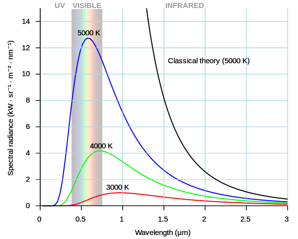
For instance, the color of a star – which varies from bluish-white and yellow to orange and red – is primarily due to its composition and effective temperature. And at all times, stars emit light which is a combination of several different wavelengths. On top of that, the color of a star can change over time.
Composition:
Different elements emit different wavelengths of electromagnetic radiation when heated. In the case of stars, his includes its main constituents (hydrogen and helium), but also the various trace elements that make it up. The color that we see is the combination of these different electromagnetic wavelengths, which are referred to as as a Planck’s curve.
Diagram illustrating Wein’s Law, which describes the emission of radiation from a black body based on its peak wavelength. Credit: Wikipedia Commons/Darth
The wavelength at which a star emits the most light is called the star’s “peak wavelength” (which known as Wien’s Law), which is the peak of its Planck curve. However, how that light appears to the human eye is also mitigated by the contributions of the other parts of its Planck curve.
In short, when the various colors of the spectrum are combined, they appear white to the naked eye. This will make the apparent color of the star appear lighter than where star’s peak wavelength falls on the color spectrum. Consider our Sun. Despite the fact that its peak emission wavelength corresponds to the green part of the spectrum, its color appears pale yellow.
A star’s composition is the result of its formation history. Ever star is born of a nebula made up of gas and dust, and each one is different. While nebulas in the interstellar medium are largely composed of hydrogen, which is the main fuel for star creation, they also carry other elements. The overall mass of the nebula, as well as the various elements that make it up, determine what kind of star will result.
The change in color these elements add to stars is not very obvious, but can be studied thanks to the method known as spectroanalysis. By examining the various wavelengths a star produces using a spectrometer, scientists are able to determine what elements are being burned inside.
Temperature and Distance:
The other major factor effecting a star’s color is its temperature. As stars increase in heat, the overall radiated energy increases, and the peak of the curve moves to shorter wavelengths. In other words, as a star becomes hotter, the light it emits is pushed further and further towards the blue end of the spectrum. As stars grow colder, the situation is reversed (see below).
A third and final factor that will effect what light a star appears to be emitting is known as the Doppler Effect. When it comes to sound, light, and other waves, the frequency can increase or decrease based on the distance between the source and the observer.
When it comes to astronomy, this effect causes the what is known as “redshift” and “blueshift” – where the visible light coming from a distant star is shifted towards the red end of the spectrum if it is moving away, and the blue end if it is moving closer.
Modern Classification:
Modern astronomy classifies stars based on their essential characteristics, which includes their spectral class (i.e. color), temperature, size, and brightness. Most stars are currently classified under the Morgan–Keenan (MK) system, which classifies stars based on temperature using the letters O, B, A, F, G, K, and M, – O being the hottest and M the coolest.
Each letter class is then subdivided using a numeric digit with 0 being hottest and 9 being coolest (e.g. O1 to M9 are the hottest to coldest stars). In the MK system, a luminosity class is added using Roman numerals. These are based on the width of certain absorption lines in the star’s spectrum (which vary with the density of the atmosphere), thus distinguishing giant stars from dwarfs.
Luminosity classes 0 and I apply to hyper- or supergiants; classes II, III and IV apply to bright, regular giants, and subgiants, respectively; class V is for main-sequence stars; and class VI and VII apply to subdwarfs and dwarf stars. There is also the Hertzsprung-Russell diagram, which relates stellar classification to absolute magnitude (i.e. intrinsic brightness), luminosity, and surface temperature.
The same classification for spectral types are used, ranging from blue and white at one end to red at the other, which is then combined with the stars Absolute Visual Magnitude (expressed as Mv) to place them on a 2-dimensional chart (see below).
The Hertzspirg-Russel diagram, showing the relation between star’s color, AM. luminosity, and temperature. Credit: astronomy.starrynight.com
On average, stars in the O-range are hotter than other classes, reaching effective temperatures of up to 30,000 K. At the same time, they are also larger and more massive, reaching sizes of over 6 and a half solar radii and up to 16 solar masses. At the lower end, K and M type stars (orange and red dwarfs) tend to be cooler (ranging from 2400 to 5700 K), measuring 0.7 to 0.96 times that of our Sun, and being anywhere from 0.08 to 0.8 as massive.
Stellar Evolution:
Stars also go through an evolutionary life cycle, during which time their sizes, temperatures and colors change. For example, when our Sun exhausts all the hydrogen in its the core, it will become unstable and collapse under its own weight. This will cause the core to heat up and get denser, causing the Sun to grow in size.
At this point, it will have left its Main Sequence phase and entered into the Red Giant Phase of its life, which (as the name would suggest) will be characterized by expansion and it becoming a deep red. When this happens, it is theorized that our Sun will expand to encompass the orbits of Mercury and even Venus.
Earth, if it survives this expansion, will be so close that it will be rendered uninhabitable. When our Sun then reaches its post-Red Giant Phase, the Sun will begin to eject mass, leaving an exposed core known as a white dwarf. This remnant will survive for trillions of years before fading to black.
This is believed to be the case with all stars that have between 0.5 to 1 Solar Mass (half, or as much mass of our Sun). The situation is slightly different when it comes to low mass stars (i.e. red dwarfs), which typically have around 0.1 Solar Masses.
It is believed that these stars can remain in their Main Sequence for some six to twelve trillion years and will not experience a Red Giant Phase. However, they will gradually increase in both temperature and luminosity, and will exist for several hundred billion more years before they eventually collapse into a white dwarf.
On the other hand, supergiant stars (up to 100 Solar Masses or more) have so much mass in their cores that they will likely experience helium ignition as soon as they exhaust their supplies of hydrogen. As such, they will likely not survive to become Red Supergiants, and will instead end their lives in a massive supernova.
To break it all down, stars vary in color depending on their chemical compositions, their respective sizes and their temperatures. Over time, as these characteristics change (as a result of them spending their fuel) many will darken and become redder, while others will explode magnificently. The more stars observe, the more we come to know about our Universe and its long, long history!
Copyright: ESA with changes to annotations by the author
This montage of photos of Comet 67P/Churyumov-Gerasimenko was taken by ESA’s Rosetta spacecraft between Jan. 31 and March 25, 2015 and shows increasing activity as the comet approached perihelion. Credit: NAVCAM /CC-BY-SA-IGO-3.0
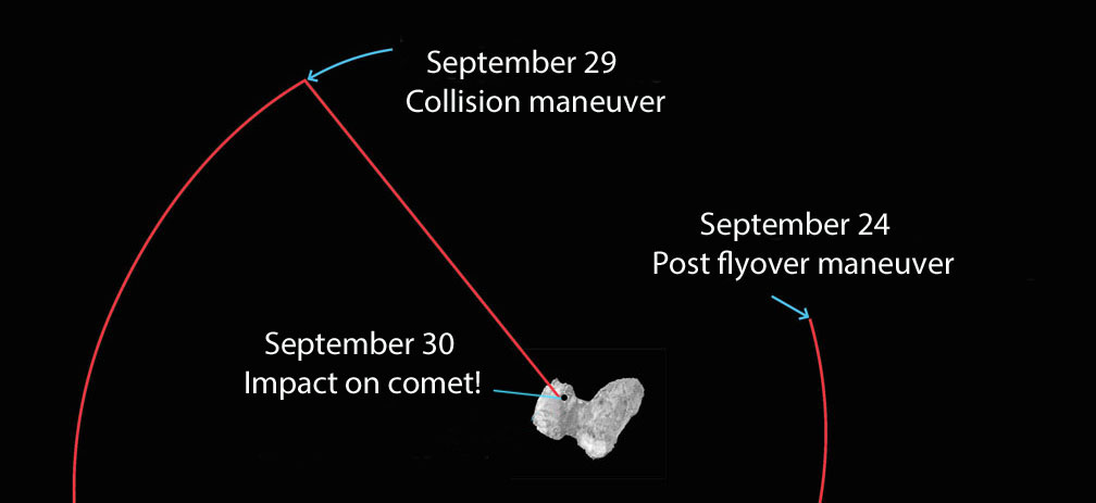
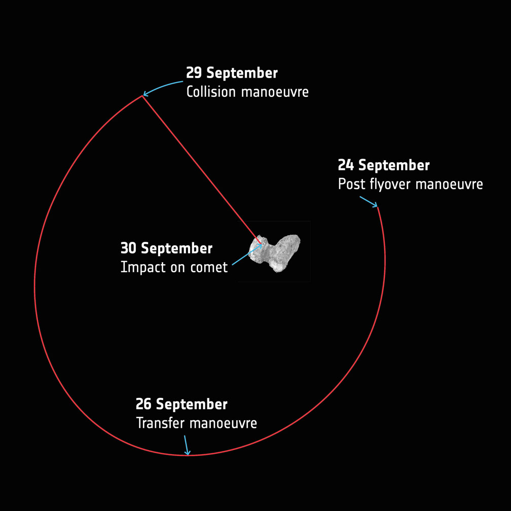
Rosetta awoke from a decade of deep-space hibernation in January 2014 and immediately got to work photographing, measuring and sampling comet 67P/C-G. On September 30 it will sleep again but this time for eternity. Mission controllers will direct the probe to impact the comet’s dusty-icy nucleus within 20 minutes of 10:40 Greenwich Time (6:40 a.m. EDT) that Friday morning. The high-resolution OSIRIS camera will be snapping pictures on the way down, but once impact occurs, it’s game over, lights out. Rosetta will power down and go silent.
A simplified overview of Rosetta’s last week of maneuvers at Comet 67P/Churyumov–Gerasimenko. Starting today (Sept. 24) the spacecraft will leave the flyover orbits and transfer towards a 16 x 23 km orbit that will be used to prepare for the final descent. The collision course maneuver will take place in the evening Sept. 29 with impact expected to occur at 10:40 GMT (6:40 a.m. EDT), which taking into account the 40 minute signal travel time between Rosetta and Earth on Sept. 30, means the confirmation would be expected at mission control at 11:20 GMT (7:20 a.m. EDT). Copyright: ESA
Nearly three years have passed since Rosetta opened its eyes on 67P, this curious, bi-lobed rubber duck of a comet just 2.5 miles (4 km) across with landscapes ranging from dust dunes to craggy peaks to enigmatic ‘goosebumps’. The mission was the first to orbit a comet and dispatch a probe, Philae, to its surface. I think it’s safe to say we learned more about what makes comets tick during Rosetta’s sojourn than in any previous mission.
So why end it? One of the big reasons is power. As Rosetta races farther and farther from the Sun, less sunlight falls on its pair of 16-meter-long solar arrays. At mid-month, the probe was over 348 million miles (560 million km) from the Sun and 433 million miles (697 million km) from Earth or nearly as far as Jupiter. With Sun-to-Rosetta mileage increasing nearly 620,000 miles (1 million km) a day, weakening sunlight can’t provide the power needed to keep the instruments running.
Rosetta’s last orbits around the comet
Rosetta’s also showing signs of age after having been in the harsh environment of interplanetary space for more than 12 years, two of them next door to a dust-spitting comet. Both factors contributed to the decision to end the mission rather than put the probe back into an even longer hibernation until the comet’s next perihelion many years away.
Since August 9, Rosetta has been swinging past the comet in a series of ever-tightening loops, providing excellent opportunities for close-up science observations. On September 5, Rosetta swooped within 1.2 miles (1.9 km) of 67P/C-G’s surface. It was hoped the spacecraft would descend as low as a kilometer during one of the later orbits as scientists worked to glean as much as possible before the show ends.
Rosetta is targeted to land at the site within this planned impact ellipse in the Ma’at region on the comet’s smaller lobe. See below for a closer view. Credit: ESA/Rosetta/NAVCAM – CC BY-SA IGO 3.0
The final of 15 close flyovers will be completed today (Sept. 24) after which Rosetta will be maneuvered from its current elliptical orbit onto a trajectory that will eventually take it down to the comet’s surface on Sept. 30.
The beginning of the end unfolds on the evening of the 29th when Rosetta spends 14 hours free-falling slowly towards the comet from an altitude of 12.4 miles (20 km) — about 4 miles higher than a typical commercial jet — all the while collecting measurements and photos that will be returned to Earth before impact. The last eye-popping images will be taken from a distance of just tens to a hundred meters away.
The landing will be a soft one, with the spacecraft touching down at walking speed. Like Philae before it, it will probably bounce around before settling into place. Mission control expects parts of the probe to break upon impact.
Taking into account the additional 40 minute signal travel time between Rosetta and Earth on the 30th, confirmation of impact is expected at ESA’s mission control in Darmstadt, Germany, within 20 minutes of 11:20 GMT (7:20 a.m. EDT). The times will be updated as the trajectory is refined. You can watch live coverage of Rosetta’s final hours on ESA TV.
ESAHangout: Preparing for Rosetta’s grand finale
“It’s hard to believe that Rosetta’s incredible 12.5 year odyssey is almost over, and we’re planning the final set of science operations, but we are certainly looking forward to focusing on analyzing the reams of data for many decades to come,” said Matt Taylor, ESA’s Rosetta project scientist.
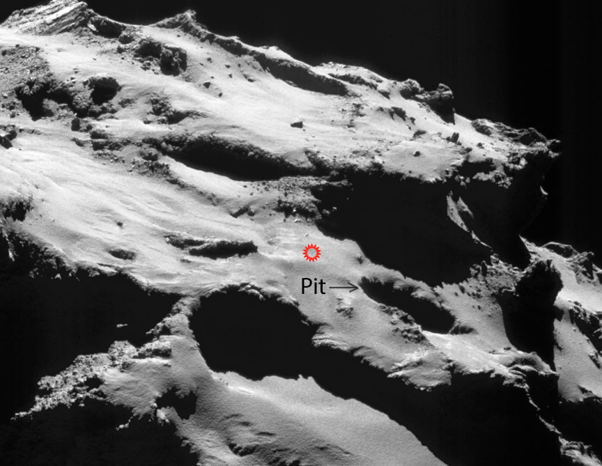
The spacecraft landing site is shown in red and located next to Deir el-Medina, a large pit (arrowed). Credit: ESA/Rosetta/NAVCAM – CC BY-SA IGO 3.0
Plans call for the spacecraft to impact the comet somewhere within an ellipse about 1,300 x 2,000 feet (600 x 400 meters) long on 67P’s smaller lobe in the region known as Ma’at. It’s home to several active pits more than 328 feet (100 meters) in diameter and 160-200 feet (50-60 meters) deep, where a number of the comet’s dust jets originate. The walls of the pits are lined with fascinating meter-sized lumpy structures called ‘goosebumps’, which scientists believe could be early ‘cometesimals’, the icy snowballs that stuck together to create the comet in the early days of our Solar System’s formation.
Close-up of a curious surface texture nicknamed ‘goosebumps’. The bumps are about 9 feet (3 meters) across and seen on very steep slopes and exposed cliff faces. They may represent the original balls of icy dust that glommed together to form comets 4.5 billion years ago. Credit: ESA/Rosetta/MPS for OSIRIS Team MPS/UPD/LAM/IAA/SSO/INTA/UPM/DASP/IDA
During free-fall, the spacecraft will target a point adjacent to a 425-foot (130 m) wide, well-defined pit that the mission team has informally named Deir el-Medina, after a structure with a similar appearance in an ancient Egyptian town of the same name. High resolution images should give us a spectacular view of these enigmatic bumps.
While we hate to see Rosetta’s mission end, it’s been a blast going for a 2-year-plus comet ride-along.