Matt Williams is a space journalist and science communicator for Universe Today and Interesting Engineering. He's also a science fiction author, podcaster (Stories from Space), and Taekwon-Do instructor who lives on Vancouver Island with his wife and family.
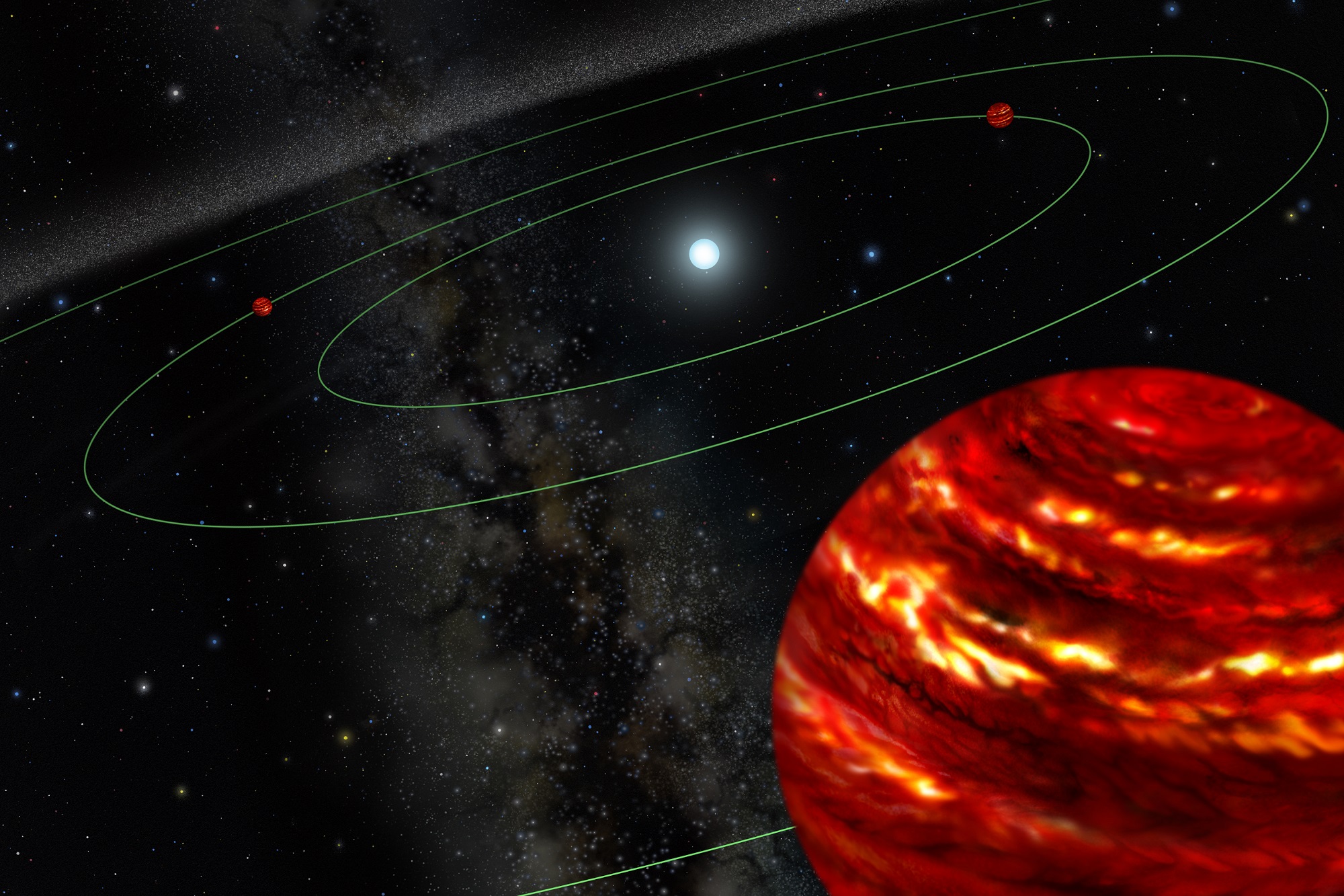
Artist's concept of the multi-planet system around HR 8799, initially discovered with Gemini North adaptive optics images. Credit: Gemini Observatory/Lynette Cook"
Located about 129 light years from Earth in the direction of the Pegasus constellation is the relatively young star system of HR 8799. Beginning in 2008, four orbiting exoplanets were discovered in this system which – alongside the exoplanet Formalhaut b – were the very first to be confirmed using the direct imaging technique. And over time, astronomer have come to believe that these four planets are in resonance with each other.
In this case, the four planets orbit their star with a 1:2:4:8 resonance, meaning that each planet’s orbital period is in a nearly precise ratio with the others in the system. This is a relatively unique phenomena, one which inspired a Jason Wang – a graduate student from the Berkeley arm of the NASA-sponsored Nexus for Exoplanet System Science (NExSS) – to produce a video that illustrates their orbital dance.
Using images obtained by the W.M. Keck Observatory over a seven year period, Wang’s video provides a glimpse of these four exoplanets in motion. As you can see below, the central star is blacked out so that the light reflecting off of its planets can be seen. And while it does not show the planets completing a full orbital period (which would take decades and even centuries) it beautifully illustrates the resonance that exists between the star’s four planets.
As Jason Wang told Universe Today via email:
“The data was obtained over 7 years from one of the 10 meter Keck telescopes by a team of astronomers (Christian Marois, Quinn Konopacky, Bruce Macintosh, Travis Barman, and Ben Zuckerman). Christian reduced each of the 7 epochs of data, to make 7 frames of data. I then made a movie by using a motion interpolation to interpolate those 7 frames into 100 frames to get a smooth video so that it’s not choppy (as if we could observe them every month from Earth).”
The images of the four exoplanets were originally captured by Dr. Christian Marois of the National Research Council of Canada’s Herzberg Institute of Astrophysics. It was in 2008 that Marois and his colleagues discovered the first three of HR 8799’s planets – HR 8799 b, c and d – using direct imaging technique. At around the same time, a team from UC Berkeley announced the discovery of Fomalhaut b, also using direct imaging.
These planets were all determined to be gas giants of similar size and mass, with between 1.2 and 1.3 times the size of Jupiter, and 7 to 10 times its mass. At the time of their discovery, HR 8799 d was believed to be the closest planet to its star, at a distance of about 27 Astronomical Units (AUs) – while the other two orbit at distances of about 42 and 68 AUs, respectively.
Image of HR 8799 (left) taken by the HST in 1998, image processed to remove scattered starlight (center), and illustration of the planetary system (right). Credit: NASA/ESA/STScI/R. Soummer
It was only afterwards that the team realized the planets had already been observed in 1998. Back then, the Hubble Space Telescope’s Near Infrared Camera and Multi-Object Spectrometer (NICMOS) had obtained light from the system that indicated the presence of planets. However, this was not made clear until after a newly-developed image-processing technique had been installed. Hence, the “pre-discovery” went unnoticed.
Further observations in 2009 and 2010 revealed the existence of fourth planet – HR 8799 e – which had an orbit placing it inside the other three. Even so, this planet is fifteen times farther from its star than the Earth is from the Sun, which results in an orbital period of about 18,000 days (49 years). The others take around 112, 225, and 450 years (respectively) to complete an orbit of HR 8799.
Ultimately, Wang decided to produce the video (which was not his first), to illustrate how exciting the search for exoplanets can be. As he put it:
“I had written this motion interpolation algorithm for another exoplanet system, Beta Pictoris b, where we see one planet on an edge-on orbit looking like it’s diving into its star (it’s actually just circling in front of it). We wanted to do the same thing for HR 8799 to bring this system to life and share our excitement in directly imaging exoplanets. I think it’s quite amazing that we have the technology to watch other worlds orbit other stars.”
In addition, the video draws attention to a star system that presents some unique opportunities for exoplanet research. Since HR 8799 was the first multi-planetary system to be directly-imaged means that astronomers can directly observe the orbits of the four planets, observe their dynamical interactions, and determine how they came to their present-day configuration.
Astronomers will also be able to take spectra of these planet’s atmospheres to study their composition, and compare this to our own Solar System’s gas giants. And since the system is really quite young (just 40 million years old), it can tell us much about the planet-formation process. Last, but not least, their wide orbits (a necessity given their size) could mean the system is less than stable.
In the future, according to Wang, astronomers will be watching to see if any planets get ejected from the system. I don’t know about you, but I would consider a video that illustrates one of HR 8799’s gas giants getting booted out of its system would be pretty inspiring too!
Using its HiRISE camera, the MRO has noted existence of tall networks of ridges on Mars that have diverse origins. Credit: NASA/JPL-Caltech/Univ. of Arizona
Mars has some impressive geological features across its cold, desiccated surface, many of which are similar to featured found here on Earth. By studying them, scientists are able to learn more about the natural history of the Red Planet, what kinds of meteorological phenomena are responsible for shaping it, and how similar our two planets are. A perfect of example of this are the polygon-ridge networks that have been observed on its surface.
One such network was recently discovered by the Mars Reconnaissance Orbiter (MRO) in the Medusae Fossae region, which straddles the planet’s equator. Measuring some 16 story’s high, this ridge network is similar to others that have been spotted on Mars. But according to a survey produced by researchers from NASA’s Jet Propulsion Laboratory, these ridges likely have different origins.
This survey, which was recently published in the journal Icarus, examined both the network found in the Medusae Fossae region and similar-looking networks in other regions of the Red Planet. These ridges (sometimes called boxwork rides), are essentially blade-like walls that look like multiple adjoining polygons (i.e. rectangles, pentagons, triangles, and similar shapes).
Shiprock, a ridge-feature in northwestern New Mexico that is 10 meters (30 feet) tall, which formed from lava filling an underground fracture that resisted erosion better than the material around it did. Credit: NASA
While similar-looking ridges can be found in many places on Mars, they do not appear to be formed by any single process. As Laura Kerber, of NASA’s Jet Propulsion Laboratory and the lead author of the survey report, explained in a NASA press release:
“Finding these ridges in the Medusae Fossae region set me on a quest to find all the types of polygonal ridges on Mars… Polygonal ridges can be formed in several different ways, and some of them are really key to understanding the history of early Mars. Many of these ridges are mineral veins, and mineral veins tell us that water was circulating underground.”
Such ridges have also been found on Earth, and appear to be the result of various processes as well. One of the most common involves lava flowing into preexisting fractures in the ground, which then survived when erosion stripped the surrounding material away. A good example of this is the Shiprock (shown above), a monadrock located in San Juan County, New Mexico.
Examples of polygon ridges on Mars include the feature known as “Garden City“, which was discovered by the Curiosity rover mission. Measuring just a few centimeters in height, these ridges appeared to be the result of mineral-laden groundwater moving through underground fissures, which led to standing mineral veins once the surrounding soil eroded away.
Mineral veins at the “Garden City” site, examined by NASA’s Curiosity Mars rover. Credit: NASA/JPL
At the other end of the scale, ridges that measure around 2 kilometers (over a mile) high have also been found. A good example of this is “Inca City“, a feature observed by the Mars Global Surveyor near Mars’ south pole. In this case, the feature is believed to be the result of underground faults (which were formed from impacts) filling with lava over time. Here too, erosion gradually stripped away the surrounding rock, exposing the standing lava rock.
In short, these features are evidence of underground water and volcanic activity on Mars. And by finding more examples of these polygon-ridges, scientists will be able to study the geological record of Mars more closely. Hence why Kerber is seeking help from the public through a citizen-science project called Planet Four: Ridges.
Established earlier this month on Zooniverse – a volunteer-powered research platform – this project has made images obtained by the MRO’s Context Camera (CTX) available to the public. Currently, this and other projects using data from CTX and HiRISE have drawn the participation of more than 150,000 volunteers from around the world.
By getting volunteers to sort through the CTX images for ridge formations, Kerber and her team hopes that previously-unidentified ones will be identified and that their relationship with other Martian features will be better understood.
Four-panel graphic showing the two pulsars, Geminga (upper left) and B0355+54 (upper right), observed by Chandra. Credit: NASA/JPL-Caltech/CXC/PSU/B.Posselt et al/N.Klingler et al/Nahks TrEhnl
Since they were first discovered in the late 1960s, pulsars have continued to fascinate astronomers. Even though thousands of these pulsing, spinning stars have been observed in the past five decades, there is much about them that continues to elude us. For instance, while some emit both radio and gamma ray pulses, others are restricted to either radio or gamma ray radiation.
However, thanks to a pair of studies from two international teams of astronomers, we may be getting closer to understanding why this is. Relying on data collected by the Chandra X-ray Observatory of two pulsars (Geminga and B0355+54), the teams was able to show how their emissions and the underlying structure of their nebulae (which resemble jellyfish) could be related.
An artist’s impression of an accreting X-ray millisecond pulsar. Credit: NASA/Goddard Space Flight Center/Dana Berry
Located 800 and 3400 light years from Earth (respectively), the Geminga and B0355+54 pulsars are quite similar. In addition to having similar rotational periods (5 times per second), they are also about the same age (~500 million years). However, Geminga emits only gamma-ray pulses while B0355+54 is one of the brightest known radio pulsars, but emits no observable gamma rays.
What’s more, their PWNs are structured quite differently. Based on composite images created using Chandra X-ray data and Spitzer infrared data, one resembles a jellyfish whose tendrils are relaxed while the other looks like a jellyfish that is closed and flexed. As Bettina Posselt – a senior research associate in the Department of Astronomy and Astrophysics at Penn State, and the lead author on the Geminga study – told Universe Today via email:
“The Chandra data resulted in two very different X-ray images of the pulsar wind nebulae around the pulsars Geminga and PSR B0355+54. While Geminga has a distinct three-tail structure, the image of PSR B0355+54 shows one broad tail with several substructures.”
In all likelihood, Geminga’s and B0355+54 tails are narrow jets emanating from the pulsar’s spin poles. These jets lie perpendicular to the donut-shaped disk (aka. a torus) that surrounds the pulsars equatorial regions. As Noel Klingler, a graduate student at the George Washington University and the author of the B0355+54 paper, told Universe Today via email:
“The interstellar medium (ISM) isn’t a perfect vacuum, so as both of these pulsars plow through space at hundreds of kilometers per second, the trace amount of gas in the ISM exerts pressure, thus pushing back/bending the pulsar wind nebulae behind the pulsars, as is shown in the images obtained by the Chandra X-ray Observatory.”
Their apparent structures appear to be due to their disposition relative to Earth. In Geminga’s case, the view of the torus is edge-on while the jets point out to the sides. In B0355+54’s case, the torus is seen face-on while the jets points both towards and away from Earth. From our vantage point, these jets look like they are on top of each other, which is what makes it look like it has a double tail. As Posselt describes it:
“Both structures can be explained with the same general model of pulsar wind nebulae. The reasons for the different images are (a) our viewing perspective, and (b) how fast and where to the pulsar is moving. In general, the observable structures of such pulsar wind nebulae can be described with an equatorial torus and polar jets. Torus and Jets can be affected (e.g., bent jets) by the “head wind” from the interstellar medium the pulsar is moving in. Depending on our viewing angle of the torus, jets and the movement of the pulsar, different pictures are detected by the Chandra X-ray observatory. Geminga is seen “from the side” (or edge-on with respect to the torus) with the jets roughly located in the plane of the sky while for B0355+54 we look almost directly to one of the poles.”
This orientation could also help explain why the two pulsars appear to emit different types of electromagnetic radiation. Basically, the magnetic poles – which are close to their spin poles – are where a pulsar’s radio emissions are believed to come from. Meanwhile, gamma rays are believed to be emitted along a pulsar’s spin equator, where the torus is located.
“The images reveal that we see Geminga from edge-on (i.e., looking at its equator) because we see X-rays from particles launched into the two jets (which are initially aligned with the radio beams), which are pointed into the sky, and not at Earth,” said Klingler. “This explains why we only see Gamma-ray pulses from Geminga. The images also indicate that we are looking at B0355+54 from a top-down perspective (i.e., above one of the poles, looking into the jets). So as the pulsar rotates, the center of the radio beam sweeps across Earth, and we detect the pulses; but the gamma-rays are launched straight out from the pulsar’s equator, so we don’t see them from B0355.”
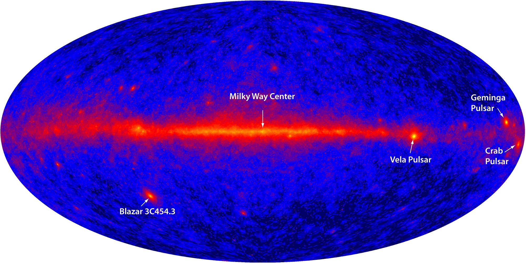
An all-sky view from the Fermi Gamma-ray Space Telescope, showing the position of Geminga in the Milky Way. Credit : NASA/DOE/International LAT Team.
“The geometrical constraints on each pulsar (where are the poles and the equator) from the pulsar wind nebulae help to explain findings regarding the radio and gamma-ray pulses of these two neutron stars,” said Posselt. “For example, Geminga appears radio-quiet (no strong radio pulses) because we don’t have a direct view to the poles and pulsed radio emission is thought to be generated in a region close to the poles. But Geminga shows strong gamma-ray pulsations, because these are not produced at the poles, but closer to the equatorial region.”
These observations were part of a larger campaign to study six pulsars that have been seen to emit gamma-rays. This campaign is being led by Roger Romani of Stanford University, with the collaboration of astronomers and researchers from GWU (Oleg Kargaltsev), Penn State University (George Pavlov), and Harvard University (Patrick Slane).
Not only are these studies shedding new light on the properties of pulsar wind nebulae, they also provide observational evidence to help astronomers create better theoretical models of pulsars. In addition, studies like these – which examine the geometry of pulsar magnetospheres – could allow astronomers to better estimate the total number of exploded stars in our galaxy.
By knowing the range of angles at which pulsars are detectable, they should be able to better estimate the amount that are not visible from Earth. Yet another way in which astronomers are working to find the celestial objects that could be lurking in humanity’s blind spots!
Artist’s impression showing the increasing effect of ram-pressure stripping in removing gas from galaxies, sending them to an early death. Credit: ICRAR/NASA/ESA/Hubble Heritage Team (STScI/AURA)
It’s what you might call a case of galactic homicide (or “galacticide”). All over the known Universe, satellite galaxies are slowly being stripped of their lifeblood – i.e. their gases. This process is responsible for halting the formation of new stars, and therefore condemning these galaxies to a relatively quick death (by cosmological standards). And for some time, astronomers have been searching for the potential culprit.
But according to a new study by a team of international researchers from the International Center for Radio Astronomy Research (ICRAR) in Australia, the answer may have to do with the hot gas galactic clusters routinely pass through. According to their study, which appeared recently in The Monthly Notices of the Royal Astronomical Society, this mechanism may be responsible for the slow death we are seeing out there.
This process is known as “ram-pressure stripping“, which occurs when the force created by the passage of galaxies through the hot plasma that lies between them is strong enough that it is able to overcome the gravitational pull of those galaxies. At this point, they lose gas, much in the same way that a planet’s atmosphere can be slowly stripped away by the effects of Solar wind.
‘Radio color’ view of the sky above the Murchison Widefield Array radio telescope, part of the International Center for Radio Astronomy Research (ICRAC). Credit: Natasha Hurley-Walker (ICRAR/Curtin)/Dr John Goldsmith/Celestial Visions.
By measuring the amount of stripping that took place within each, they deduced that the extent to which a galaxy was stripped of its essential gases had much to do with the mass of its dark matter halo. For some time, astronomers have believed that galaxies are embedded in clouds of this invisible mass, which is believed to make up 27% of the known Universe.
“During their lifetimes, galaxies can inhabit halos of different sizes, ranging from masses typical of our own Milky Way to halos thousands of times more massive. As galaxies fall through these larger halos, the superheated intergalactic plasma between them removes their gas in a fast-acting process called ram-pressure stripping. You can think of it like a giant cosmic broom that comes through and physically sweeps the gas from the galaxies.”
The Arecibo Observatory in Puerto Rico, where the Arecibo Legacy Fast ALFA Survey is conducted. Credit: egg.astro.cornell.edu
This stripping is what deprives satellites galaxies of their ability to form new stars, which ensures that the stars they have enter their red giant phase. This process, which results in a galaxy populated by cooler stars, makes them that much harder to see in visible light (though still detectable in the infrared band). Quietly, but quickly, these galaxies become cold, dark, and fade away.
Already, astronomers were aware of the effects of ram-pressure stripping of galaxies in clusters, which boast the largest dark matter halos found in the Universe. But thanks to their study, they are now aware that it can affect satellite galaxies as well. Ultimately, this shows that the process of ram-pressure stripping is more prevalent than previously thought.
As Dr. Barbara Catinella, an ICRAR researcher and co-author on the study, put it:
“Most galaxies in the Universe live in these groups of between two and a hundred galaxies. We’ve found this removal of gas by stripping is potentially the dominant way galaxies are quenched by their surroundings, meaning their gas is removed and star formation shuts down.”
Another major way in which galaxies die is known as “strangulation”, which occurs when a galaxy’s gas is consumed faster than it can be replenished. However, compared to ram-pressure stripping, this process is very gradual, taking billions of years rather than just tens of millions – very fast on a cosmological time scale. Also, this process is more akin to a galaxy suffering from famine after outstripping its food source, rather than homicide.
Another cosmological mystery solved, and one that has crime-drama implications no less!
JAXA's H-IIA Launch Vehicle taking off from the Tanegashima Space Center. Credit: Wikipedia Commons/NARITA Masahiro
The Japanese Aerospace Exploration Agency (JAXA) has accomplished some impressive things over the years. Between 2003 (when it was formed) and 2016, the agency has launched multiple satellites – ranging from x-ray and infrared astronomy to lunar and Venus atmosphere exploration probes – and overseen Japan’s participation in the International Space Station.
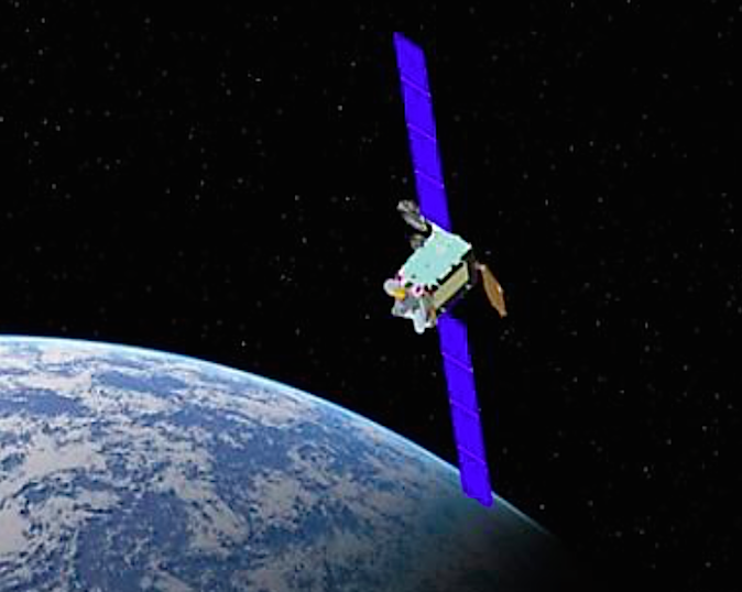
But in what is an historic mission – and a potentially controversial one – JAXA recently launched the first of three X-band defense communication satellites into orbit. By giving the Japanese Self-Defense Forces the ability to relay communications and commands to its armed forces, this satellite (known as DSN 2) represents an expansion of Japan’s military capability.
The launch took place on January 24th at 4:44 pm Japan Standard Time (JST) – or 0744 Greenwich Mean Time (GMT) – with the launch of a H-IIA rocket from Tanegashima Space Center. This was the thirty-second successful flight of the launch vehicle, and the mission was completed with the deployment of the satellite in Low-Earth Orbit – 35,000 km; 22,000 mi above the surface of the Earth.
Artist’s concept of a Japanese X-band military communications satellite. Credit: Japanese Ministry of Defense
Shortly after the completion of the mission, JAXA issued a press release stating the following:
“At 4:44 p.m., (Japan Standard Time, JST) January 24, Mitsubishi Heavy Industries, Ltd. and JAXA launched the H-IIA Launch Vehicle No. 32 with X-band defense communication satellite-2* on board. The launch and the separation of the satellite proceeded according to schedule. Mitsubishi Heavy Industries, Ltd. and JAXA express appreciation for the support in behalf of the successful launch. At the time of the launch the weather was fine, at 9 degrees Celsius, and the wind speed was 7.1 meters/second from the NW.”
This launch is part of a $1.1 billion program by the Japanese Defense Ministry to develop X-band satellite communications for the Japan Self-Defense Forces (JSDF). With the overall goal of deploying three x-band relay satellites into geostationary orbit, its intended purpose is to reduce the reliance of Japan’s military (and those of its allies) on commercial and international communications providers.
While this may seem like a sound strategy, it is a potential source of controversy in that it may skirt the edge of what is constitutionally permitted in Japan. In short, deploying military satellites is something that may be in violation of Japan’s post-war agreements, which the nation committed to as part of its surrender to the Allies. This includes forbidding the use of military force as a means of solving international disputes.
An H-2A rocket, Japan’s primary large-scale launch vehicle. Credit: JAXA
It also included placing limitations on its Self-Defense Forces so they would not be capable of independent military action. As is stated in Article 9 of the Constitution of Japan (passed in 1947):
“(1) Aspiring sincerely to an international peace based on justice and order, the Japanese people forever renounce war as a sovereign right of the nation and the threat or use of force as means of settling international disputes.
(2) In order to accomplish the aim of the preceding paragraph, land, sea, and air forces, as well as other war potential, will never be maintained. The right of belligerency of the state will not be recognized.”
However, since 2014, the Japanese government has sought to reinterpret Article 9 of the constitution, claiming that it allows the JSDF the freedom to defend other allies in case of war. This move has largely been in response to mounting tensions with North Korea over its development of nuclear weapons, as well as disputes with China over issues of sovereignty in the South China Sea.
This interpretation has been the official line of the Japanese Diet since 2015, as part of a series of measures that would allow the JSDF to provide material support to allies engaged in combat internationally. This justification, which claims that Japan and its allies would be endangered otherwise, has been endorsed by the United States. However, to some observers, it may very well be interpreted as an attempt by Japan to re-militarize.
In the coming weeks, the DSN 2 spacecraft will use its on-board engine to position itself in geostationary orbit, roughly 35,800 km (22,300 mi) above the equator. Once there, it will commence a final round of in-orbit testing before commencing its 15-year term of service.
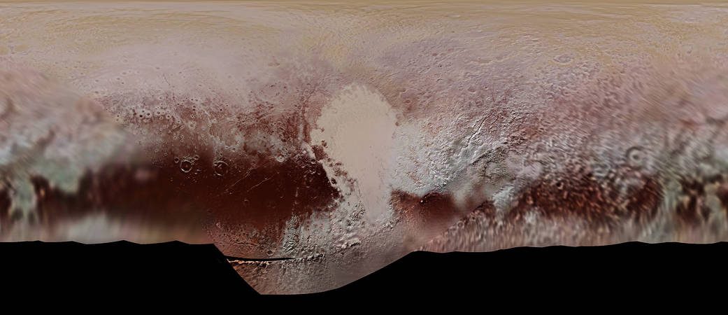
Color mosaic map of Pluto's surface, created from the New Horizons many photographs. Credit: NASA/JHUAPL/SwRI
On July 14th, 2015, the New Horizons mission made history by conducting the first flyby of Pluto. This represented the culmination of a nine year journey, which began on January 19th, 2006 – when the spacecraft was launched from the Cape Canaveral Air Force Station. And before the mission is complete, NASA hopes to send the spacecraft to investigate objects in the Kuiper Belt as well.
To mark the 11th anniversary of the spacecraft’s launch, members of the New Horizons team took part in panel a discussion hosted by the Johns Hopkins University Applied Physics Laboratory (JHUAPL) located in Laurel, Maryland. The event was broadcasted on Facebook Live, and consisted of team members speaking about the highlights of the mission and what lies ahead for the NASA spacecraft.
The live panel discussion took place on Thursday, Sept. 19th at 4 p.m. EST, and included Jim Green and Alan Stern – the director the Planetary Science Division at NASA and the principle investigator (PI) of the New Horizons mission, respectively. Also in attendance was Glen Fountain and Helene Winters, New Horizons‘ project managers; and Kelsi Singer, the New Horizons co-investigator.
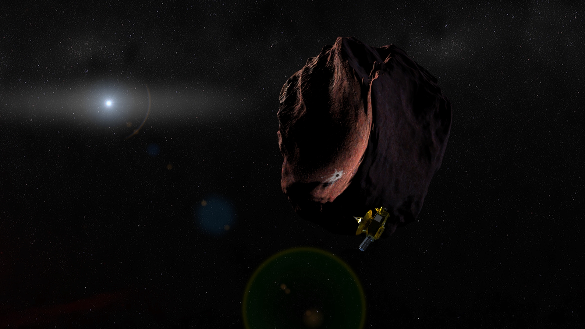
Artist’s concept of the New Horizons spacecraft encountering a Kuiper Belt object, part of an extended mission after the spacecraft’s July 2015 Pluto flyby. Credits: NASA/JHUAPL/SwRI
In the course of the event, the panel members responded to questions and shared stories about the mission’s greatest accomplishments. Among them were the many, many high-resolution photographs taken by the spacecraft’s Ralph and Long Range Reconnaissance Imager (LORRI) cameras. In addition to providing detailing images of Pluto’s surface features, they also allowed for the creation of the very first detailed map of Pluto.
Though Pluto is not officially designated as a planet anymore – ever since the XXVIth General Assembly of the International Astronomical Union, where Pluto was designated as a “dwarf planet” – many members of the team still consider it to be the ninth planet of the Solar System. Because of this, New Horizons‘ historic flyby was of particular significance.
As Principle Investigator Alan Stern – from the Southwestern Research Institute (SwRI) – explained in an interview with Inverse, the first phase of humanity’s investigation of the Solar System is now complete. “What we did was we provided the capstone to the initial exploration of the planets,” he said. “All nine have been explored with New Horizons finishing that task.”
Other significant discoveries made by the New Horizons mission include Pluto’s famous heart-shaped terrain – aka. Sputnik Planum. This region turned out to be a young, icy plain that contains water ice flows adrift on a “sea” of frozen nitrogen. And then there was the discovery of the large mountain and possible cryovolcano located at the tip of the plain – named Tombaugh Regio, (in honor of Pluto’s discovered, Clyde Tombaugh).
New Horizons path from the inner Solar System to Pluto and the Kuiper Belt. Credit: NASA/JHUAPL
The mission also revealed further evidence of geological activity and cryovolcanism, the presence of hyrdocarbon clouds on Pluto, and conducted the very first measurements of how Pluto interacts with solar wind. All told, over 50 gigabits of data were collected by New Horizons during its encounter and flyby with Pluto. And the detailed map which resulted from it did a good job of capturing all this complexity and diversity. As Stern explained:
“That really blew away our expectations. We did not think that a planet the size of North America could be as complex as Mars or even Earth. It’s just tons of eye candy. This color map is the highest resolution we will see until another spacecraft goes back to Pluto.”
After making its historic flyby of Pluto, the New Horizons team requested that the mission receive an extension to 2021 so that it could explore Kuiper Belt Objects (KBOs). This extension was granted, and for the first part of the Kuiper Belt Extended Mission (KEM), the spacecraft will perform a close flyby of the object known as 2014 MU69.
This remote KBO – which is estimated to be between 25 – 45 km (16-28 mi) in diameter – was one of two objects identified as potential targets for research, and the one recommended by the New Horizons team. The flyby, which is expected to take place in January of 2019, will involve the spacecraft taking a series of photographs on approach, as well as some pictures of the object’s surface once it gets closer.
Before the extension ends in 2021, it will continue to send back information on the gas, dust and plasma conditions in the Kuiper Belt. Clearly, we are not finished with the New Horizons mission, and it is not finished with us!
No immediate plausibility issues with this picture, since the speedometer says 0.8c. Getting it past 1.0c is where it gets tricky.
It’s always a welcome thing to learn that ideas that are commonplace in science fiction have a basis in science fact. Cryogenic freezers, laser guns, robots, silicate implants… and let’s not forget the warp drive! Believe it or not, this concept – alternately known as FTL (Faster-Than-Light) travel, Hyperspace, Lightspeed, etc. – actually has one foot in the world of real science.
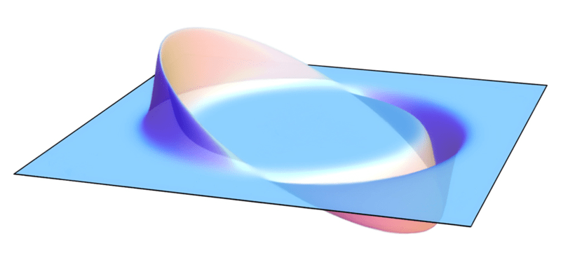
In physics, it is what is known as the Alcubierre Warp Drive. On paper, it is a highly speculative, but possibly valid, solution of the Einstein field equations, specifically how space, time and energy interact. In this particular mathematical model of spacetime, there are features that are apparently reminiscent of the fictional “warp drive” or “hyperspace” from notable science fiction franchises, hence the association.
Background:
Since Einstein first proposed the Special Theory of Relativity in 1905, scientists have been operating under the restrictions imposed by a relativistic universe. One of these restrictions is the belief that the speed of light is unbreakable and hence, that there will never be such a thing as FTL space travel or exploration.
Visualization of a warp field, according to the Alcubierre Drive. Credit: AllenMcC
Even though subsequent generations of scientists and engineers managed to break the sound barrier and defeat the pull of the Earth’s gravity, the speed of light appeared to be one barrier that was destined to hold. But then, in 1994, a Mexican physicist by the name of Miguel Alcubierre came along with proposed method for stretching the fabric of space-time in way which would, in theory, allow FTL travel to take pace.
Concept:
To put it simply, this method of space travel involves stretching the fabric of space-time in a wave which would (in theory) cause the space ahead of an object to contract while the space behind it would expand. An object inside this wave (i.e. a spaceship) would then be able to ride this region, known as a “warp bubble” of flat space.
This is what is known as the “Alcubierre Metric”. Interpreted in the context of General Relativity, the metric allows a warp bubble to appear in a previously flat region of spacetime and move away, effectively at speeds that exceed the speed of light. The interior of the bubble is the inertial reference frame for any object inhabiting it.
Since the ship is not moving within this bubble, but is being carried along as the region itself moves, conventional relativistic effects such as time dilation would not apply. Hence, the rules of space-time and the laws of relativity would not be violated in the conventional sense.
Artist’s concept of a spacecraft using an Alcubierre Warp Drive. Credit: NASA
One of the reasons for this is because this method would not rely on moving faster than light in the local sense, since a light beam within this bubble would still always move faster than the ship. It is only “faster than light” in the sense that the ship could reach its destination faster than a beam of light that was traveling outside the warp bubble.
Difficulties:
However, there is are few problems with this theory. For one, there are no known methods to create such a warp bubble in a region of space that would not already contain one. Second, assuming there was a way to create such a bubble, there is not yet any known way of leaving once inside it. As a result, the Alcubierre drive (or metric) remains in the category of theory at this time.
Mathematically, it can be represented by the following equation: ds2= – (a2 – BiBi) dt2 + 2Bi dxi dt + gijdxi dxj, where a is the lapse function that gives the interval of proper time between nearby hypersurfaces, Biis the shift vector that relates the spatial coordinate systems on different hypersurfaces and gij is a positive definite metric on each of the hypersurfaces.
Attempts at Development:
In 1996, NASA founded a research project known as the Breakthrough Propulsion Physics Project (BPP) to study various spacecraft proposals and technologies. In 2002, the project’s funding was discontinued, which prompted the founder – Marc G. Millis – and several members to create the Tau Zero Foundation. Named after the famous novel of the same name by Poul Anderson, this organization is dedicated to researching interstellar travel.
In 2012, NASA’s Advanced Propulsion Physics Laboratory (aka. Eagleworks) announced that they had began conducting experiments to see if a “warp drive” was in fact possible. This included developing an interferometer to detect the spatial distortions produced by the expanding and contracting space-time of the Alcubierre metric.
The team lead – Dr. Harold Sonny White – described their work in a NASA paper titled Warp Field Mechanics 101. He also explained their work in NASA’s 2012 Roundup publication:
“We’ve initiated an interferometer test bed in this lab, where we’re going to go through and try and generate a microscopic instance of a little warp bubble. And although this is just a microscopic instance of the phenomena, we’re perturbing space time, one part in 10 million, a very tiny amount… The math would allow you to go to Alpha Centauri in two weeks as measured by clocks here on Earth. So somebody’s clock onboard the spacecraft has the same rate of time as somebody in mission control here in Houston might have. There are no tidal forces, no undue issues, and the proper acceleration is zero. When you turn the field on, everybody doesn’t go slamming against the bulkhead, (which) would be a very short and sad trip.”
In 2013, Dr. White and members of Eagleworks published the results of their 19.6-second warp field test under vacuum conditions. These results, which were deemed to be inconclusive, were presented at the 2013 Icarus Interstellar Starship Congress held in Dallas, Texas.
When it comes to the future of space exploration, some very tough questions seem unavoidable. And questions like “how long will it take us to get the nearest star?” seem rather troubling when we don’t make allowances for some kind of hypervelocity or faster-than-light transit method. How can we expect to become an interstellar species when all available methods with either take centuries (or longer), or will involve sending a nanocraft instead?
At present, such a thing just doesn’t seem to be entirely within the realm of possibility. And attempts to prove otherwise remain unsuccessful or inconclusive. But as history has taught us, what is considered to be impossible changes over time. Someday, who knows what we might be able to accomplish? But until then, we’ll just have to be patient and wait on future research.
According to data from NASA and the NOAA, 2016 was the hottest year on record yet again. Credit: NASA
The reality of Climate Change has become painfully apparent in recent years, thanks to extended droughts in places like California, diminishing water tables around the world, rising tides, and coastal storms of increasing intensity and frequency. But perhaps the most measurable trend is the way that average global temperatures have kept rising year after year.
And this has certainly been the case for the year of 2016. According to independent analyses provided by NASA’s Goddard Institute for Space Studies (GISS) and the National Oceanic and Atmospheric Agency (NOAA), 2016 was the warmest year since modern record keeping began in 1880. This represents a continuation of a most alarming trend, where 16 of the 17 warmest years on record have occurred since 2001.
Based in New York, GISS conducts space and Earth sciences research, in support of the Goddard Space Flight Center’s (GSFC) Sciences and Exploration Directorate. Since its establishment in 1961, the Institute has conducted valuable research on Earth’s structure and atmosphere, the Earth-Sun relationship, and the structure and atmospheres of other planets in the Solar System.
Monthly temperature anomalies with base 1980-2015, superimposed on a 1980-2015 mean seasonal cycle. Credit: NASA/GISS/Schmidt
Their early studies of Earth and other solar planets using data collected by satellites, space probes, and landers eventually led to GISS becoming a leading authority on atmospheric modeling. Similarly, the NOAA efforts to monitor atmospheric conditions and weather in the US since 1970s has led to them becoming a major scientific authority on Climate Change.
Together, the two organizations looked over global temperature data for the year of 2016 and came to the same conclusion. Based on their assessments, GISS determined that globally-averaged surface temperatures in 2016 were 0.99 °C (1.78 °F) warmer than the mid-20th century mean. As GISS Director Gavin Schmidt put it, these findings should silence any doubts about the ongoing nature of Global Warming:
“2016 is remarkably the third record year in a row in this series. We don’t expect record years every year, but the ongoing long-term warming trend is clear.”
The NOAA’s findings were similar, with an average temperature of 14.83 °C (58.69 °F) being reported for 2016. This surpassed last year’s record by about 0.004 °C (0.07 °F), and represents a change of around 0.94 °C (1.69 F) above the 20th century average. The year began with a boost, thanks to El Nino; and for the eight consecutive months that followed (January to August) the world experienced record temperatures.
This represents a consistent change since 2001, where average global temperatures have increased, leading to of the 16 warmest years on record since 1880 in a row. In addition, on five separate occasions during this period, the annual global temperature was record-breaking – in 2005, 2010, 2014, 2015, and 2016, respectively.
Land and ocean global temperatures in 2013 from both NASA and NOAA. Credit: NASA.
With regards to the long-term trend, average global temperatures have increased by about 1.1° Celsius (2° Fahrenheit) since 1880. This too represents a change, since the rate of increase was placed at 0.8° Celsius (1.4° Fahrenheit) back in 2014. Two-thirds of this warming has occurred since 1975, which coincides with a period of rapid population growth, industrialization, and increased consumption of fossil fuels.
And while there is always a degree of uncertainty when it comes to atmospheric and temperature modelling, owing to the fact that the location of measuring stations and practices change over time, NASA indicated that they were over 95% certain of these results. As such, there is little reason to doubt them, especially since they are consistent with what is at this point a very well-documented trend.
To see an animated graph of average global temperature increases since 1880, click here. To see the full data set and learn about the methods employed by GISS, click here.
And be sure to check out this NASA video that shows these changes on a global map:
Portrait of Max Planck (c. 1930). Credit: Smithsonian Libraries
Imagine if you will that your name would forever be associated with a groundbreaking scientific theory. Imagine also that your name would even be attached to a series of units, designed to performs measurements for complex equations. Now imagine that you were German who lived through two World Wars, won the Nobel Prize for physics, and outlived many of your children.
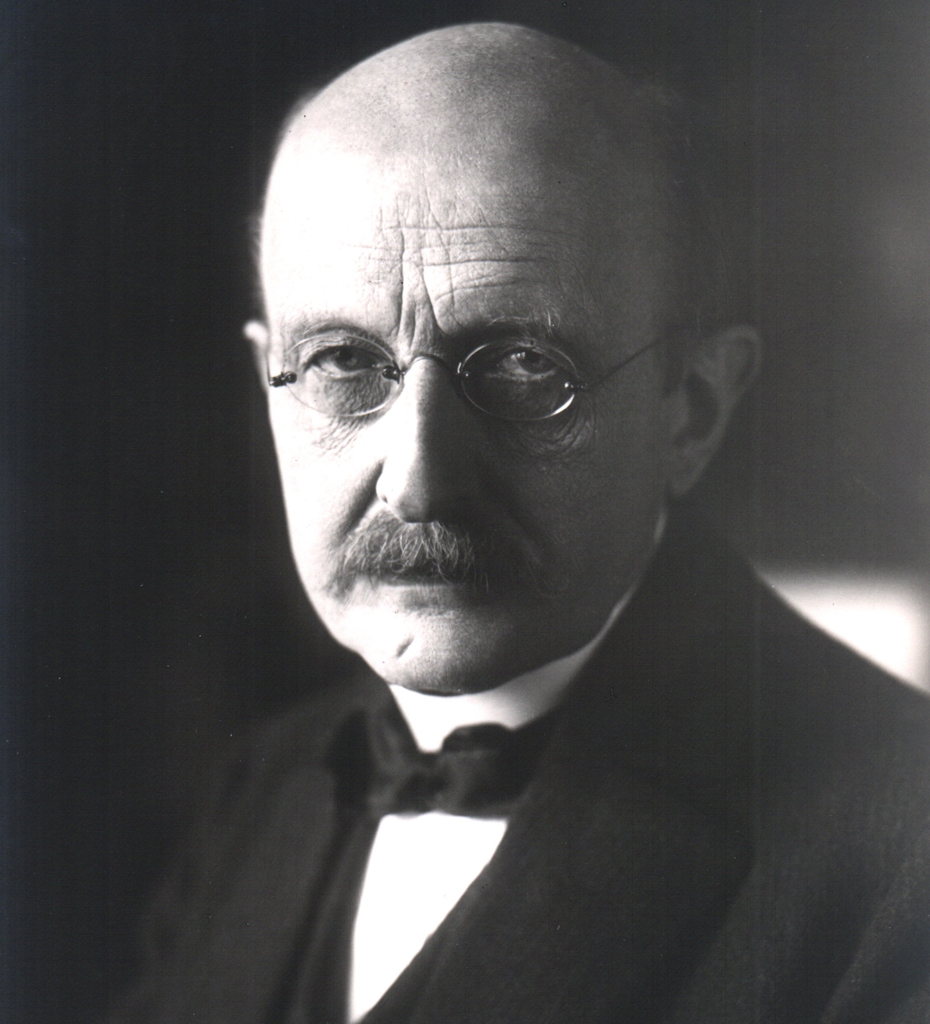
If you can do all that, then you might know what it was like to be Max Planck, the German physicist and founder of quantum theory. Much like Galileo, Newton, and Einstein, Max Planck is regarded as one of the most influential and groundbreaking scientists of his time, a man whose discoveries helped to revolutionized the field of physics. Ironic, considering that when he first embarked on his career, he was told there was nothing new to be discovered!
Early Life and Education:
Born in 1858 in Kiel, Germany, Planck was a child of intellectuals, his grandfather and great-grandfather both theology professors and his father a professor of law, and his uncle a judge. In 1867, his family moved to Munich, where Planck enrolled in the Maximilians gymnasium school. From an early age, Planck demonstrated an aptitude for mathematics, astronomy, mechanics, and music.
Illustration of Friedrich Wilhelms University, with the statue of Frederick the Great (ca. 1850). Credit: Wikipedia Commons/A. Carse
He graduated early, at the age of 17, and went on to study theoretical physics at the University of Munich. In 1877, he went on to Friedrich Wilhelms University in Berlin to study with physicists Hermann von Helmholtz. Helmholtz had a profound influence on Planck, who he became close friends with, and eventually Planck decided to adopt thermodynamics as his field of research.
In October 1878, he passed his qualifying exams and defended his dissertation in February of 1879 – titled “On the second law of thermodynamics”. In this work, he made the following statement, from which the modern Second Law of Thermodynamics is believed to be derived: “It is impossible to construct an engine which will work in a complete cycle, and produce no effect except the raising of a weight and cooling of a heat reservoir.”
For a time, Planck toiled away in relative anonymity because of his work with entropy (which was considered a dead field). However, he made several important discoveries in this time that would allow him to grow his reputation and gain a following. For instance, his Treatise on Thermodynamics, which was published in 1897, contained the seeds of ideas that would go on to become highly influential – i.e. black body radiation and special states of equilibrium.
With the completion of his thesis, Planck became an unpaid private lecturer at the Freidrich Wilhelms University in Munich and joined the local Physical Society. Although the academic community did not pay much attention to him, he continued his work on heat theory and came to independently discover the same theory of thermodynamics and entropy as Josiah Willard Gibbs – the American physicist who is credited with the discovery.
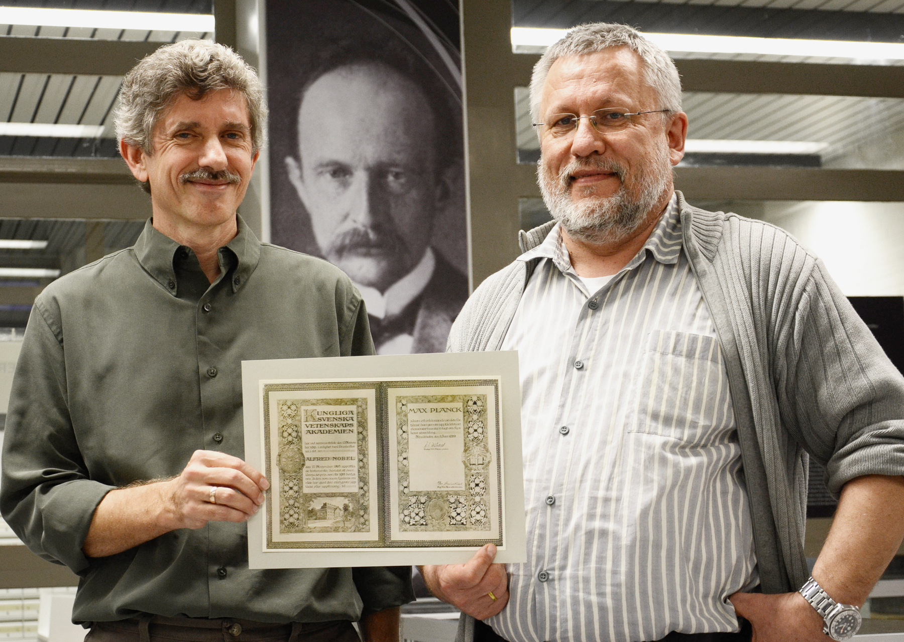
Professors Michael Bonitz and Frank Hohmann, holding a facsimile of Planck’s Nobel prize certificate, which was given to the University of Kiel in 2013. Credit and Copyright: CAU/Schimmelpfennig
In 1885, the University of Kiel appointed Planck as an associate professor of theoretical physics, where he continued his studies in physical chemistry and heat systems. By 1889, he returned to Freidrich Wilhelms University in Berlin, becoming a full professor by 1892. He would remain in Berlin until his retired in January 1926, when he was succeeded by Erwin Schrodinger.
Black Body Radiation:
It was in 1894, when he was under a commission from the electric companies to develop better light bulbs, that Planck began working on the problem of black-body radiation. Physicists were already struggling to explain how the intensity of the electromagnetic radiation emitted by a perfect absorber (i.e. a black body) depended on the bodies temperature and the frequency of the radiation (i.e., the color of the light).
In time, he resolved this problem by suggesting that electromagnetic energy did not flow in a constant form but rather in discreet packets, i.e. quanta. This came to be known as the Planck postulate, which can be stated mathematically as E = hv – where E is energy, v is the frequency, and h is the Planck constant. This theory, which was not consistent with classical Newtonian mechanics, helped to trigger a revolution in science.
A deeply conservative scientists who was suspicious of the implications his theory raised, Planck indicated that he only came by his discovery reluctantly and hoped they would be proven wrong. However, the discovery of Planck’s constant would prove to have a revolutionary impact, causing scientists to break with classical physics, and leading to the creation of Planck units (length, time, mass, etc.).
From left to right: W. Nernst, A. Einstein, M. Planck, R.A. Millikan and von Laue at a dinner given by von Laue in Berlin, 1931. Credit: Wikipedia Commons
Quantum Mechanics:
By the turn of the century another influential scientist by the name of Albert Einstein made several discoveries that would prove Planck’s quantum theory to be correct. The first was his theory of photons (as part of his Special Theory of Relativity) which contradicted classical physics and the theory of electrodynamics that held that light was a wave that needed a medium to propagate.
The second was Einstein’s study of the anomalous behavior of specific bodies when heated at low temperatures, another example of a phenomenon which defied classical physics. Though Planck was one of the first to recognize the significance of Einstein’s special relativity, he initially rejected the idea that light could made up of discreet quanta of matter (in this case, photons).
However, in 1911, Planck and Walther Nernst (a colleague of Planck’s) organized a conference in Brussels known as the First Solvav Conference, the subject of which was the theory of radiation and quanta. Einstein attended, and was able to convince Planck of his theories regarding specific bodies during the course of the proceedings. The two became friends and colleagues; and in 1914, Planck created a professorship for Einstein at the University of Berlin.
During the 1920s, a new theory of quantum mechanics had emerged, which was known as the “Copenhagen interpretation“. This theory, which was largely devised by German physicists Neils Bohr and Werner Heisenberg, stated that quantum mechanics can only predict probabilities; and that in general, physical systems do not have definite properties prior to being measured.
Photograph of the first Solvay Conference in 1911 at the Hotel Metropole in Brussels, Belgium. Credit: International Solvay Institutes/Benjamin Couprie
This was rejected by Planck, however, who felt that wave mechanics would soon render quantum theory unnecessary. He was joined by his colleagues Erwin Schrodinger, Max von Laue, and Einstein – all of whom wanted to save classical mechanics from the “chaos” of quantum theory. However, time would prove that both interpretations were correct (and mathematically equivalent), giving rise to theories of particle-wave duality.
World War I and World War II:
In 1914, Planck joined in the nationalistic fervor that was sweeping Germany. While not an extreme nationalist, he was a signatory of the now-infamous “Manifesto of the Ninety-Three“, a manifesto which endorsed the war and justified Germany’s participation. However, by 1915, Planck revoked parts of the Manifesto, and by 1916, he became an outspoken opponent of Germany’s annexation of other territories.
After the war, Planck was considered to be the German authority on physics, being the dean of Berlin Universit, a member of the Prussian Academy of Sciences and the German Physical Society, and president of the Kaiser Wilhelm Society (KWS, now the Max Planck Society). During the turbulent years of the 1920s, Planck used his position to raise funds for scientific research, which was often in short supply.
The Nazi seizure of power in 1933 resulted in tremendous hardship, some of which Planck personally bore witness to. This included many of his Jewish friends and colleagues being expelled from their positions and humiliated, and a large exodus of Germans scientists and academics.
Entrance of the administrative headquarters of the Max Planck Society in Munich. Credit: Wikipedia Commons/Maximilian Dörrbecker
Planck attempted to persevere in these years and remain out of politics, but was forced to step in to defend colleagues when threatened. In 1936, he resigned his positions as head of the KWS due to his continued support of Jewish colleagues in the Society. In 1938, he resigned as president of the Prussian Academy of Sciences due to the Nazi Party assuming control of it.
Despite these evens and the hardships brought by the war and the Allied bombing campaign, Planck and his family remained in Germany. In 1945, Planck’s son Erwin was arrested due to the attempted assassination of Hitler in the July 20th plot, for which he was executed by the Gestapo. This event caused Planck to descend into a depression from which he did not recover before his death.
Death and Legacy:
Planck died on October 4th, 1947 in Gottingen, Germany at the age of 89. He was survived by his second wife, Marga von Hoesslin, and his youngest son Hermann. Though he had been forced to resign his key positions in his later years, and spent the last few years of his life haunted by the death of his eldest son, Planck left a remarkable legacy in his wake.
In recognition for his fundamental contribution to a new branch of physics he was awarded the Nobel Prize in Physics in 1918. He was also elected to the Foreign Membership of the Royal Society in 1926, being awarded the Society’s Copley Medal in 1928. In 1909, he was invited to become the Ernest Kempton Adams Lecturer in Theoretical Physics at Columbia University in New York City.
The Max Planck Medal, issued by the German Physical Society in recognition of scientific contributions. Credit: dpg-physik.de
He was also greatly respected by his colleagues and contemporaries and distinguished himself by being an integral part of the three scientific organizations that dominated the German sciences- the Prussian Academy of Sciences, the Kaiser Wilhelm Society, and the German Physical Society. The German Physical Society also created the Max Planck Medal, the first of which was awarded into 1929 to both Planck and Einstein.
The Max Planck Society was also created in the city of Gottingen in 1948 to honor his life and his achievements. This society grew in the ensuing decades, eventually absorbing the Kaiser Wilhelm Society and all its institutions. Today, the Society is recognized as being a leader in science and technology research and the foremost research organization in Europe, with 33 Nobel Prizes awarded to its scientists.
In 2009, the European Space Agency (ESA) deployed the Planck spacecraft, a space observatory which mapped the Cosmic Microwave Background (CMB) at microwave and infra-red frequencies. Between 2009 and 2013, it provided the most accurate measurements to date on the average density of ordinary matter and dark matter in the Universe, and helped resolve several questions about the early Universe and cosmic evolution.
Planck shall forever be remembered as one of the most influential scientists of the 20th century. Alongside men like Einstein, Schrodinger, Bohr, and Heisenberg (most of whom were his friends and colleagues), he helped to redefine our notions of physics and the nature of the Universe.
An artist’s impression of what Mars might have looked like with water. Credit: ESO/M. Kornmesser
For some time, scientists have suspected that life may have existed on Mars in the deep past. Owing to the presence of a thicker atmosphere and liquid water on its surface, it is entirely possible that the simplest of organisms might have begun to evolve there. And for those looking to make Mars a home for humanity someday, it is hoped that these conditions (i.e favorable to life) could be recreated again someday.
But as it turns out, there are some terrestrial organisms that could survive on Mars as it is today. According to a recent study by a team of researchers from the Arkansas Center for Space and Planetary Sciences (ACSPS) at the University of Arkansas, four species of methanogenic microorganisms have shown that they could withstand one of the most severe conditions on Mars, which is its low-pressure atmosphere.
Methanogenic organisms that were found in samples of deep volcanic rocks along the Columbia River and in Idaho Falls. Credit: NASA
To put it simply, Methanogens are ancient group of organisms that are classified as archaea, a species of microorganism that do not require oxygen and can therefore survive in what we consider to be “extreme environments”. On Earth, methanogens are common in wetlands, ocean environments, and even in the digestive tracts of animals, where they consume hydrogen and carbon dioxide to produce methane as a metabolic byproduct.
And as several NASA missions have shown, methane has also been found in the atmosphere of Mars. While the source of this methane has not yet been determined, it has been argued that it could be produced by methanogens living beneath the surface. As Rebecca Mickol, an astrobiologist at the ACSPS and the lead author of the study, explained:
“One of the exciting moments for me was the detection of methane in the Martian atmosphere. On Earth, most methane is produced biologically by past or present organisms. The same could possibly be true for Mars. Of course, there are a lot of possible alternatives to the methane on Mars and it is still considered controversial. But that just adds to the excitement.”
As part of the ongoing effort to understand the Martian environment, scientists have spent the past 20 years studying if four specific strains of methanogen – Methanothermobacter wolfeii, Methanosarcina barkeri, Methanobacterium formicicum, Methanococcus maripaludis – can survive on Mars. While it is clear that they could endure the low-oxygen and radiation (if underground), there is still the matter of the extremely low air-pressure.
Graduate students Rebecca Mickol and Navita Sinha prepare to load methanogens into the Pegasus Chamber housed in W.M. Keck Laboratory. Credit: University of Arkansas
With help from the NASA Exobiology & Evolutionary Biology Program (part of NASA’s Astrobiology Program), which issued them a three-year grant back in 2012, Mickol and her team took a new approach to testing these methanogens. This included placing them in a series of test tubes and adding dirt and fluids to simulate underground aquifers. They then fed the samples hydrogen as a fuel source and deprived them of oxygen.
The next step was subjecting the microorganisms to pressure conditions analogues to Mars to see how they might hold up. For this, they relied on the Pegasus Chamber, an instrument operated by the ACSPS in their W.M. Keck Laboratory for Planetary Simulations. What they found was that the methanogens all survived exposure to pressures of 6 to 143 millibars for periods of between 3 and 21 days.
This study shows that certain species of microorganisms are not dependent on a the presence of a dense atmosphere for their survival. It also shows that these particular species of methanogens could withstand periodic contact with the Martian atmosphere. This all bodes well for the theories that Martian methane is being produced organically – possibly in subsurface, wet environments.
This is especially good news in light of evidence provided by NASA’s HiRISE instrument concerning Mars’ recurring slope lineae, which pointed towards a possible connection between liquid water columns on the surface and deeper levels in the subsurface. If this should prove to be the case, then organisms being transported in the water column would be able to withstand the changing pressures during transport.
The possible ways methane might get into Mars’ atmosphere, ranging from subsurface microbes and weathering of rock and stored methane ice called a clathrate. Ultraviolet light can work on surface materials to produce methane as well as break it apart into other molecules (. Credit: NASA/JPL-Caltech/SAM-GSFC/Univ. of Michigan
The next step, according to Mickol is to see how these organisms can stand up to temperature. “Mars is very, very cold,” she said, “often getting down to -100ºC (-212ºF) at night, and sometimes, on the warmest day of the year, at noon, the temperature can rise above freezing. We’d run our experiments just above freezing, but the cold temperature would limit evaporation of the liquid media and it would create a more Mars-like environment.”
Scientists have suspected for some time that life may still be found on Mars, hiding in recesses and holes that we have yet to peek into. Research that confirms that it can indeed exist under Mars’ present (and severe) conditions is most helpful, in that it allows us to narrow down that search considerably.
In the coming years, and with the deployment of additional Mars missions – like NASA’s Interior Exploration using Seismic Investigations, Geodesy and Heat Transport (InSight) lander, which is scheduled for launch in May of next year – we will be able to probe deeper into the Red Planet. And with sample return missions on the horizon – like the Mars 2020 rover – we may at last find some direct evidence of life on Mars!


