magnetic field Archives

August 4, 2017February 7, 2021 by Matt Williams

Bad News For Proxima b: An Earth-Like Atmosphere Might Not Survive There

Artist’s impression of Proxima b, which was discovered using the Radial Velocity method. Credit: ESO/M. Kornmesser

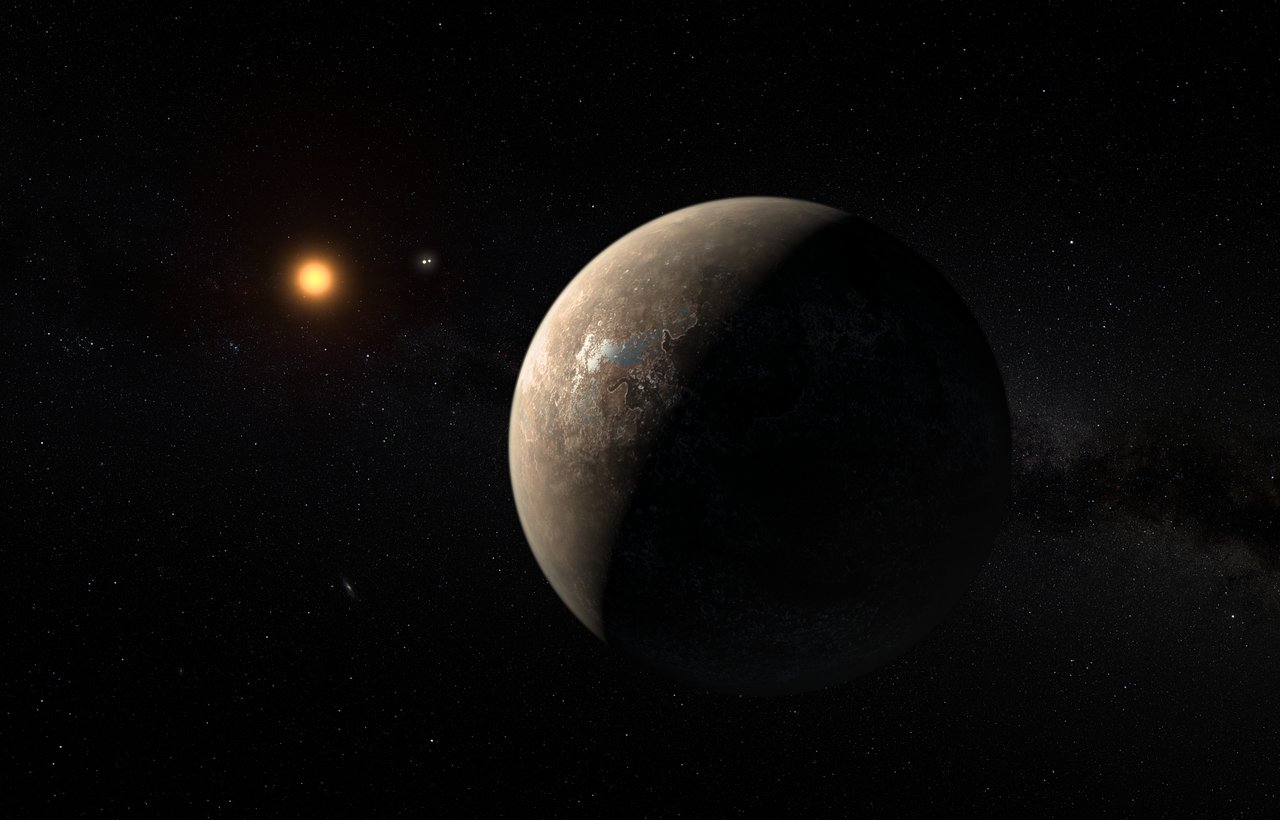
Back in of August of 2016, the existence of an Earth-like planet right next door to our Solar System was confirmed. To make matters even more exciting, it was confirmed that this planet orbits within its star’s habitable zone too. Since that time, astronomers and exoplanet-hunters have been busy trying to determine all they can about this rocky planet, known as Proxima b. Foremost on everyone’s mind has been just how likely it is to be habitable.

However, numerous studies have emerged since that time that indicate that Proxima b, given the fact that it orbits an M-type (red dwarf), would have a hard time supporting life. This was certainly the conclusion reached in a new study led by researchers from NASA’s Goddard Space Flight Center. As they showed, a planet like Proxima b would not be able to retain an Earth-like atmosphere for very long.

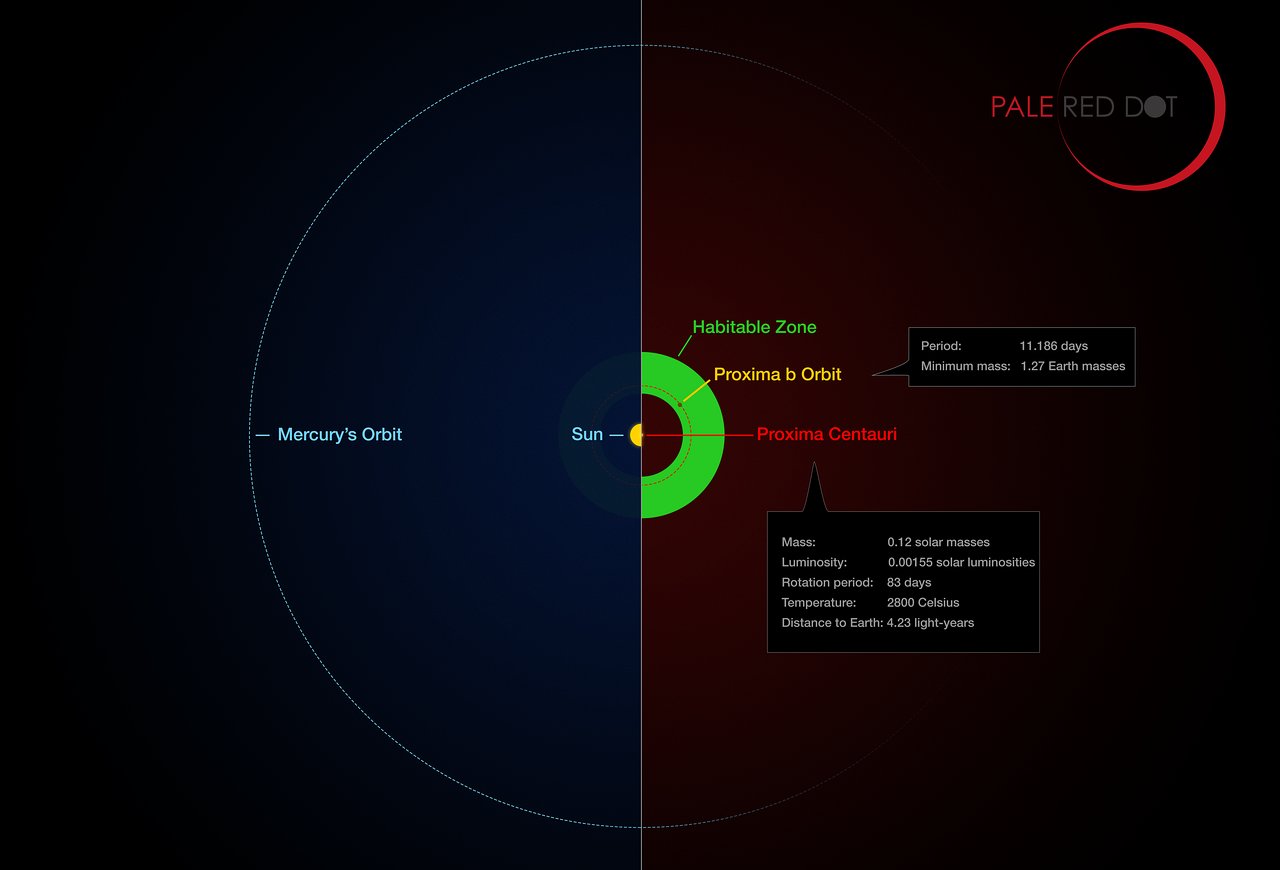
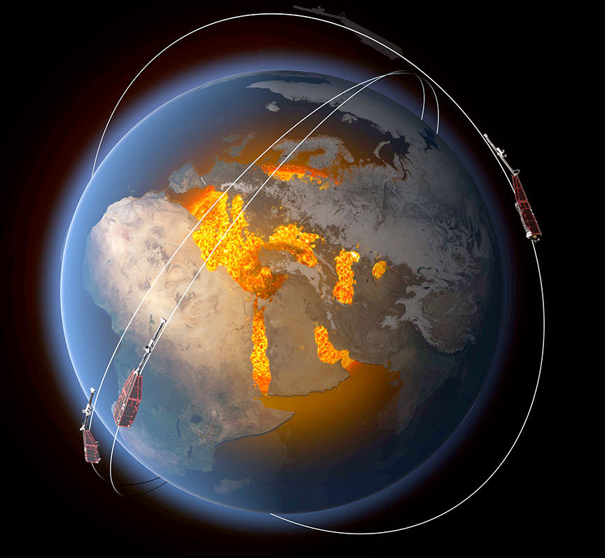
Red dwarf stars are the most common in the Universe, accounting for an estimated 70% of stars in our galaxy alone. As such, astronomers are naturally interested in knowing just how likely they are at supporting habitable planets. And given the distance between our Solar System and Proxima Centauri – 4.246 light years – Proxima b is considered ideal for studying the habitability of red dwarf star systems.

*This infographic compares the orbit of the planet around Proxima Centauri (Proxima b) with the same region of the Solar System. Credit: Pale Red Dot*

On top of all that, the fact that Proxima b is believed to be similar in size and composition to Earth makes it an especially appealing target for research. The study was led by Dr. Katherine Garcia-Sage of NASA’s Goddard Space Flight Center and the Catholic University of America in Washington, DC. As she told Universe Today via email:

“So far, not many Earth-sized exoplanets have been found orbiting in the temperate zone of their star. That doesn’t mean they don’t exist – larger planets are found more often because they are easier to detect – but Proxima b is of interest because it’s not only Earth-sized and at the right distance from its star, but it’s also orbiting the closest star to our Solar System.”

For the sake of determining if Proxima b could be habitable, the research team sought to address the chief concerns facing rocky planets that orbit red dwarf stars. These include the planet’s distance from its stars, the variability of red dwarfs, and the presence (or absence) of magnetic fields. Distance is of particular importance since habitable zones (aka. temperate zones) around red dwarfs are much closer and tighter.

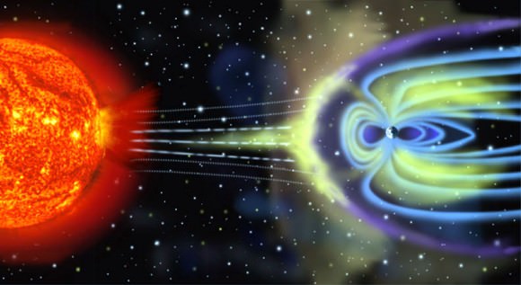
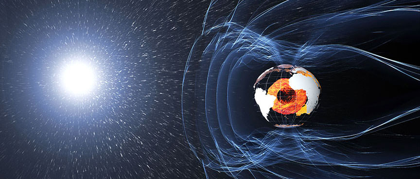
“Red dwarfs are cooler than our own Sun, so the temperate zone is closer to the star than Earth is to the Sun,” said Dr. Garcia-Sage. “But these stars may be very magnetically active, and being so close to a magnetically active star means that these planets are in a very different space environment than what the Earth experiences. At those distances from the star, the ultraviolet and x-ray radiation may be quite large. The stellar wind may be stronger. There could be stellar flares and energetic particles from the star that ionize and heat the upper atmosphere.”

*At one time, Mars had a magnetic field similar to Earth, which prevented its atmosphere from being stripped away. Credit: NASA*

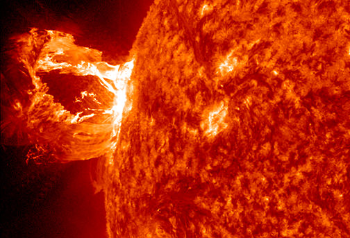
In addition, red dwarf stars are known for being unstable and variable in nature when compared to our Sun. As such, planets orbiting in close proximity would have to contend with flare ups and intense solar wind, which could gradually strip away their atmospheres. This raises another important aspect of exoplanet habitability research, which is the presence of magnetic fields.

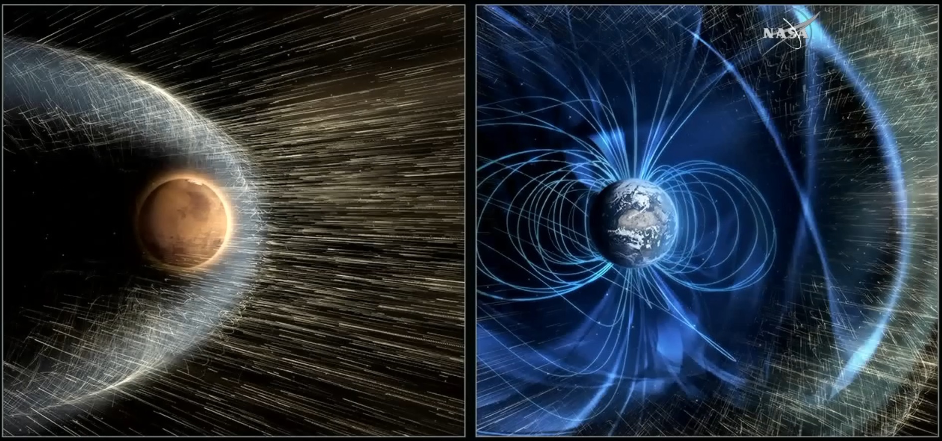
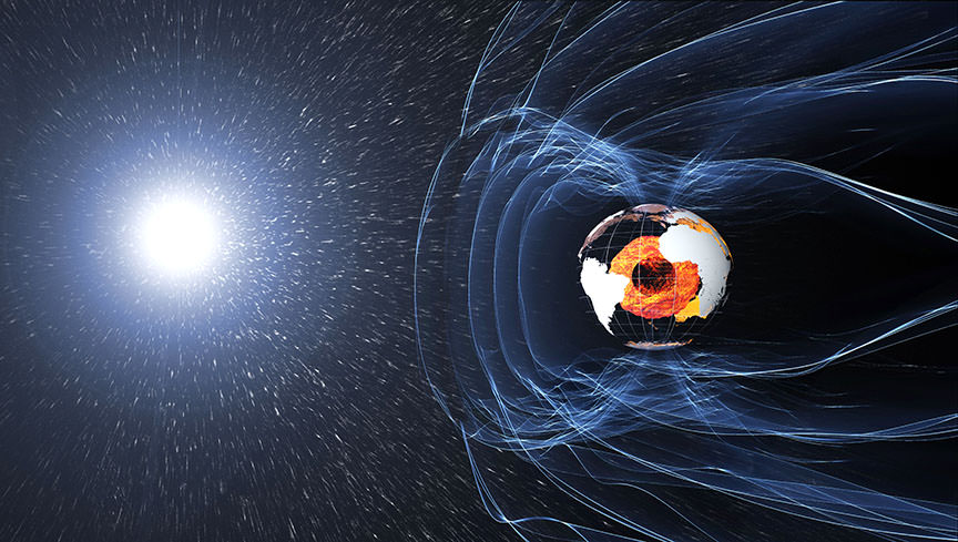
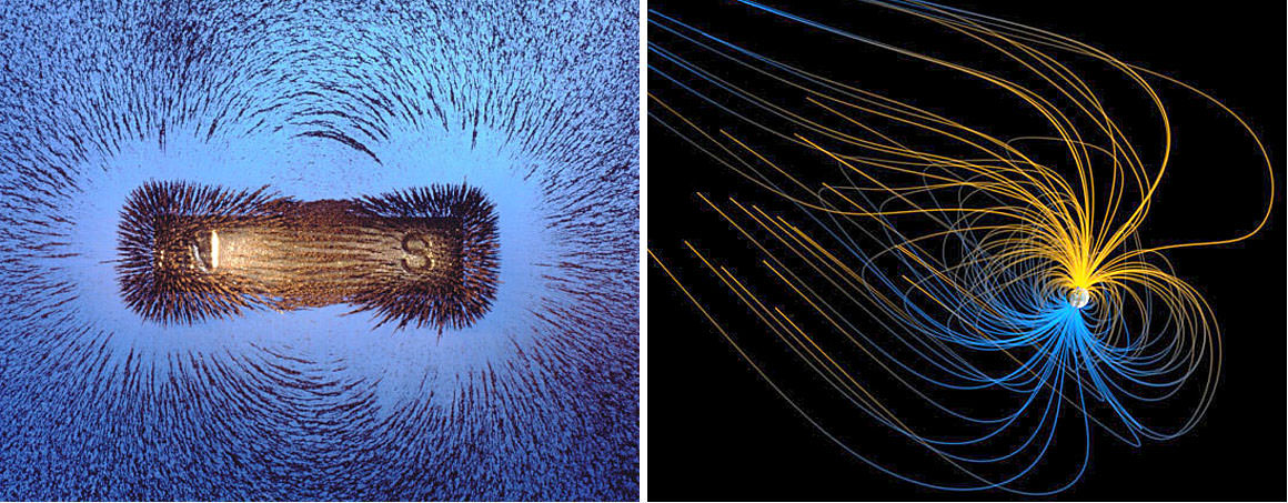
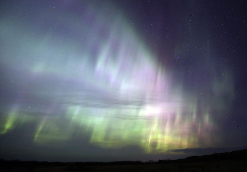
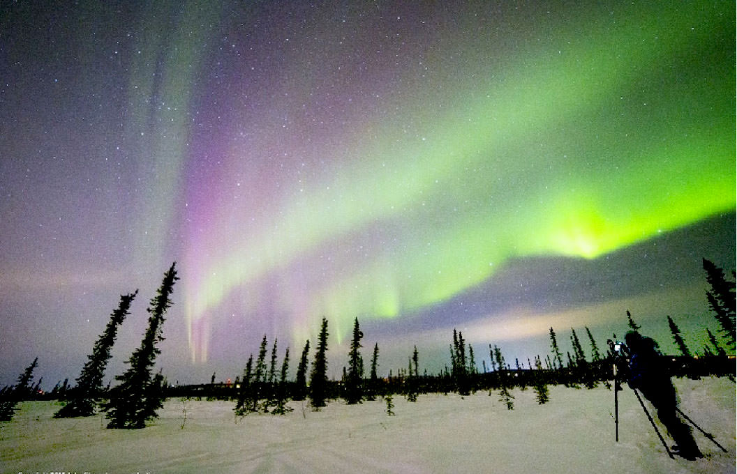
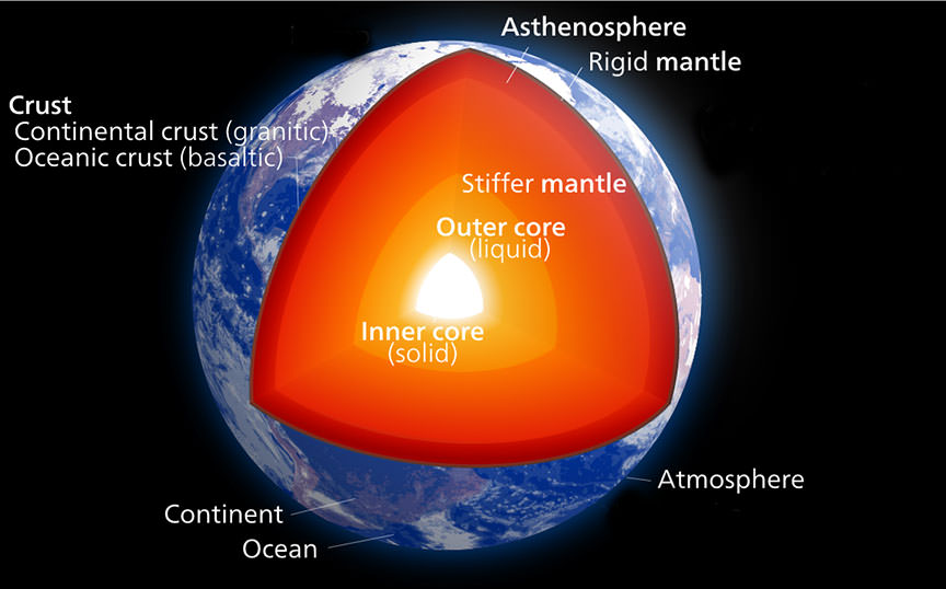
To put it simply, Earth’s atmosphere is protected by a magnetic field that is driven by a dynamo effect in its outer core. This “magnetosphere” has prevented solar wind from stripping our atmosphere away, thus giving life a chance to emerge and evolve. In contrast, Mars lost its magnetosphere roughly 4.2 billion years ago, which led to its atmosphere being depleted and its surface becoming the cold, desiccated place it is today.

To test Proxima b’s potential habitability and capacity to retain liquid surface water, the team therefore assumed the presence of an Earth-like atmosphere and a magnetic field around the planet. They then accounted for the enhanced radiation coming from Proxima b. This was provided by the Harvard Smithsonian Center for Astrophysics (CfA), where researchers determined the ultraviolet and x-ray spectrum of Proxima Centauri for this project.

From all of this, they constructed models that began to calculate the rate of atmospheric loss, using Earth’s atmosphere as a template. As Dr. Garcia-Sage explained:

“At Earth, the upper atmosphere is ionized and heated by ultraviolet and x-ray radiation from the Sun. Some of these ions and electrons escape from the upper atmosphere at the north and south poles. We have a model that calculates how fast the upper atmosphere is lost through these processes (it’s not very fast at Earth)… We then used that radiation as the input for our model and calculated a range of possible escape rates for Proxima Centauri b, based on varying levels of magnetic activity.”

Artist’s impression of the surface of the planet Proxima b orbiting the red dwarf star Proxima Centauri. The double star Alpha Centauri AB is visible to the upper right of Proxima itself. Credit: ESO

What they found was not very encouraging. In essence, Proxima b would not be able to retain an Earth-like atmosphere when subjected to Proxima Centauri’s intense radiation, even with the presence of a magnetic field. This means that unless Proxima b has had a very different kind of atmospheric history than Earth, it is most likely a lifeless ball of rock.

However, as Dr. Garcia-Sage put it, there are other factors to consider which their study simply can’t account for:

“We found that atmospheric losses are much stronger than they are at Earth, and the for high levels of magnetic activity that we expect at Proxima b, the escape rate was fast enough that an entire Earth-like atmosphere could be lost to space. That doesn’t take into account other things like volcanic activity or impacts with comets that might be able to replenish the atmosphere, but it does mean that when we’re trying to understand what processes shaped the atmosphere of Proxima b, we have to take into account the magnetic activity of the star. And understanding the atmosphere is an important part of understanding whether liquid water could exist on the surface of the planet and whether life could have evolved.”

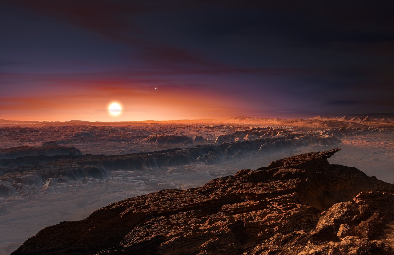
So it’s not all bad news, but it doesn’t inspire a lot of confidence either. Unless Proxima b is a volcanically-active planet and subject to a lot of cometary impacts, it is not likely be temperate, water-bearing world. Most likely, its climate will be analogous to Mars – cold, dry, and with water existing mostly in the form of ice. And as for indigenous life emerging there, that’s not too likely either.

These and other recent studies have painted a rather bleak picture about the habitability of red dwarf star systems. Given that these are the most common types of stars in the known Universe, the statistical likelihood of finding a habitable planet beyond our Solar System appears to be dropping. Not exactly good news at all for those hoping that life will be found out there within their lifetimes!

But it is important to remember that what we can say definitely at this point about extra-solar planets is limited. In the coming years and decades, next-generation missions – like the James Webb Space Telescope (JWST) and the Transiting Exoplanet Survey Satellite (TESS) – are sure to paint a more detailed picture. In the meantime, there’s still plenty of stars in the Universe, even if most of them are extremely far away!

Further Reading: The Astrophysical Journal Letters

June 13, 2017June 13, 2017 by Fraser Cain

Flying Into the Sun? NASA’s Parker Solar Probe Mission

If you’ve read enough of our articles, you know I’ve got an uneasy alliance with the Sun. Sure, it provides the energy we need for all life on Earth. But, it’s a great big ongoing thermonuclear reaction, and it’s right there! As soon as we get fusion, Sun, in like, 30 years or so, I tell you, we’ll be the ones laughing.

But to be honest, we still have so many questions about the Sun. For starters, we don’t fully understand the solar wind blasting out of the Sun. This constant wind of charged particles is constantly blowing out into space, but sometimes it’s stronger, and sometimes it’s weaker.

What are the factors that contribute to the solar wind? And as you know, these charged particles are not healthy for the human body, or for our precious electronics. In fact, the Sun occasionally releases enormous blasts that can damage our satellites and electrical grids.

How can we predict the intensity so that we can be better prepared for dangerous solar storms? Especially the Carrington-class events that might take down huge portions of our modern society.

Perhaps the biggest mystery with the Sun is the temperature of its corona. The surface of the Sun is hot, like 5,500 degrees Celsius. But if you rise up into the atmosphere of the Sun, into its corona, the temperature jumps beyond a million degrees.

The list of mysteries is long. And to start understanding what’s going on, we’ll need to get much much closer to the Sun.

Good news, NASA has a new mission in the works to do just that.

The Parker Solar Probe logo. Credit: NASA/JHUAPL

The mission is called the Parker Solar Probe. Actually, last week, it was called the Solar Probe Plus, but then NASA renamed it, and that reminded me to do a video on it.

It’s pretty normal for NASA to rename their spacecraft, usually after a dead astronomer/space scientist, like Kepler, Chandra, etc. This time, though, they renamed it for a legendary solar astronomer Eugene Parker, who developed much of our modern thinking on the Sun’s solar wind. Parker just turned 90 and this is the first time NASA has named it after someone living.

Anyway, back to the spacecraft.

The mission is due to launch in early August 2018 on a Delta IV Heavy, so we’re still more than a year away at this point. When it does, it’ll carry the spacecraft on a very unusual trajectory through the inner Solar System.

The problem is that the Sun is actually a very difficult place to reach. In fact, it’s the hardest place to get to in the entire Solar System.

Remember that the Earth is traveling around the Sun at a velocity of 30 km/s. That’s almost three times the velocity it takes to get into orbit. That’s a lot of velocity.

In order to be able to get anywhere near the Sun, the probe needs to shed velocity. And in order to do this, it’s going to use gravitational slingshots with Venus. We’ve talked about gravitational slingshots in the past, and how you can use them to speed up a spacecraft, but you can actually do the reverse.

The Parker Solar Probe will fall down into Venus’ gravity well, and give orbital velocity to Venus. This will put it on a new trajectory which takes it closer to the Sun. It’ll do a total of 7 flybys in 7 years, each of which will tweak its trajectory and shed some of that orbital momentum.

Parker Solar Probe's trajectory including Venus flybys. Credit: NASA/JHUAPL — Parker Solar Probe’s trajectory including Venus flybys. Credit: NASA/JHUAPL

You know, trying to explain orbital maneuvering is tough. I highly recommend that you try out Kerbal Space Program. I’ve learned more about orbital mechanics by playing that game for a few months than I have in almost 2 decades of space journalism. Go ahead, try to get to the Sun, I challenge you.

Anyway, with each Venus flyby, the Parker Solar Probe will get closer and closer to the Sun, well within the orbit of Mercury. Far closer than any spacecraft has ever gotten to the Sun. At its closest point, it’ll only be 5.9 million kilometers from the Sun. Just for comparison, the Earth orbits at an average distance of about 150 million kilometers. That’s close.

And over the course of its entire mission, the spacecraft is expected to make a total of 24 complete orbits of the Sun, analyzing that plasma ball from every angle.

The orbit is also highly elliptical, which means that it’s going really really fast at its closest point. Almost 725,000 km/h.

In order to withstand the intense temperatures of being this close to the Sun, NASA has engineered the Parker Solar Probe to shed heat. It’s equipped with an 11.5 cm-thick shield made of carbon-composite. For that short time it spends really close to the Sun, the spacecraft will keep the shield up, blocking that heat from reaching the rest of its instruments.

And it’s going to get hot. We’re talking about more than 1,300 degrees Celsius, which is about 475 times as much energy as a spacecraft receives here on Earth. In the outer Solar System, the problem is that there just isn’t enough energy to power solar panels. But where Parker is going, there’s just too much energy.

Now we’ve talked about the engineering difficulties of getting a spacecraft this close to the Sun, let’s talk about the science.

Coronal holes are regions in the sun’s atmosphere or corona where solar plasma can stream directly into space. Often a hole will a couple rotations, inciting repeat auroras approximately every 4 weeks. Credit: NASA

The biggest question astronomers are looking to solve is, how does the corona get so hot. The surface is 5,500 Celsius. As you get farther away from the Sun, you’d expect the temperature to go down. And it certainly does once you get as far as the orbit of the Earth.

But the Sun’s corona, or its outer atmosphere, extends millions of kilometers into space. You can see it during a solar eclipse as this faint glow around the Sun. Instead of dropping, the temperature rises to more than a million degrees.

What could be causing this? There are a couple of ideas. Plasma waves pushed off the Sun could bunch up and release their heat into the corona. You could also get the crisscrossing of magnetic field lines that create mini-flares within the corona, heating it up.

The second great mystery is the solar wind, the stream of charged protons and electrons coming from the Sun. Instead of a constant blowing wind, it can go faster or slower. And when the speed changes, the contents of the wind change too.

There’s the slow wind, that goes a mere 1.1 million km/h and seems to emanate from the Sun’s equatorial regions. And then the fast wind, which seems to be coming out of coronal holes, cooler parts in the Sun’s corona, and can be going at 2.7 million km/h.

Why does the solar wind speed change? Why does its consistency change?

Parker Solar Probe's instruments. Credit: NASA/JHUAPL — Parker Solar Probe’s instruments. Credit: NASA/JHUAPL

The Parker Solar Probe is equipped with four major instruments, each of which will gather data from the Sun and its environment.

The FIELDS experiment will measure the electric and magnetic fields and waves around the Sun. We know that much of the Sun’s behavior is driven by the complex interaction between charged plasma in the Sun. In fact, many physicists agree that magnetohydrodynamics is easily one of the most complicated fields you can get into.

Integrated Science Investigation of the Sun, or ISOIS (which I suspect needs a renaming) will measure the charged particles streaming off the Sun, during regular solar activity and during dangerous solar storms. Can we get any warning before these events occur, giving astronauts more time to protect themselves?

Wide-field Imager for Solar PRobe or WISPR is its telescope and camera. It’s going to be taking close up, high resolution images of the Sun and its corona that will blow our collective minds… I hope. I mean, if it’s just a bunch of interesting data and no pretty pictures, it’s going to be hard to make cool videos showcasing the results of the mission. You hear me NASA, we want pictures and videos. And science, sure.

And then the Solar Wind Electrons Alphas and Protons Investigation, or SWEAP, will measure type, velocity, temperature and density of particles around the Sun, to help us understand the environment around it.

One interesting side note, the spacecraft will be carrying a tiny chip on board with photos of Eugene Parker and a copy of his original 1958 paper explaining the Sun’s solar wind.

The Parker Solar Probe orbiting the Sun. Credit: NASA/JHUAPL

I know we’re still more than a year away from liftoff, and several years away before the science data starts pouring in. But you’ll be hearing more and more about this mission shortly, and I’m pretty excited about what it’s going to accomplish. So stay tuned, and once the science comes in, I’m sure you’ll hear plenty more about it.

April 15, 2017April 28, 2017 by Matt Williams

Dynamo At Moon’s Heart Once Powered Magnetic Field Equal To Earth’s

The #MemoriesInDNA project intends to create an archive of human knowledge which will be sent to the Moon. Credit and copyright: John Brimacombe.

When the Apollo astronauts returned to Earth, they came bearing 380.96 kilograms (839.87 lb) of Moon rocks. From the study of these samples, scientists learned a great deal about the Moon’s composition, as well as its history of formation and evolution. For example, the fact that some of these rocks were magnetized revealed that roughly 3 billion years ago, the Moon had a magnetic field.

Much like Earth, this field would have been the result of a dynamo effect in the Moon’s core. But until recently, scientists have been unable to explain how the Moon could maintain such a dynamo effect for so long. But thanks to a new study by a team of scientists from the Astromaterials Research and Exploration Science (ARES) Division at NASA’s Johnson Space Center, we might finally have a answer.

To recap, the Earth’s magnetic core is an integral part of what keeps our planet habitable. Believed to be the result of a liquid outer core that rotates in the opposite direction as the planet, this field protects the surface from much of the Sun’s radiation. It also ensures that our atmosphere is not slowly stripped away by solar wind, which is what happened with Mars.

*The Moon rocks returned by the Apollo 11 astronauts. Credit: NASA*

For the sake of their study, which was recently published in the journal Earth and Planetary Science Letters, the ARES team sought to determine how a molten, churning core could generate a magnetic field on the Moon. While scientists have understood how the Moon’s core could have powered such a field in the past, they have been unclear as to how it could have been maintained it for such a long time.

Towards this end, the ARES team considered multiple lines of geochemical and geophysical evidence to put constraints on the core’s composition. As Kevin Righter, the lead of the JSC’s high pressure experimental petrology lab and the lead author of the study, explained in a NASA press release:

“Our work ties together physical and chemical constraints and helps us understand how the moon acquired and maintained its magnetic field – a difficult problem to tackle for any inner solar system body. We created several synthetic core compositions based on the latest geochemical data from the moon, and equilibrated them at the pressures and temperatures of the lunar interior.”

Specifically, the ARES scientists conducted simulations of how the core would have evolved over time, based on varying levels of nickel, sulfur and carbon content. This consisted of preparing powders or iron, nickel, sulfur and carbon and mixing them in the proper proportions – based on recent analyses of Apollo rock samples.

*Artist concept illustration of the internal structure of the moon. Credit: NOAJ*

Once these mixtures were prepared, they subjected them to heat and pressure conditions consistent with what exists at the Moon’s core. They also varied these temperatures and pressures based on the possibility that the Moon underwent changes in temperature during its early and later history – i.e. hotter during its early history and cooler later on.

What they found was that a lunar core composed of iron/nickel that had a small amount of sulfur and carbon – specifically 0.5% sulfur and 0.375% carbon by weight – fit the bill. Such a core would have a high melting point and would have likely started crystallizing early in the Moon’s history, thus providing the necessary heat to drive the dynamo and power a lunar magnetic field.

This field would have eventually died out after heat flow led the core to cool, thus arresting the dynamo effect. Not only do these results provide an explanation for all the paleomagnetic and seismic data we currently have on the Moon, it is also consistent with everything we know about the Moon’s geochemical and geophysical makeup.

Prior to this, core models tended to place the Moon’s sulfur content much higher. This would mean that it had a much lower melting point, and would have meant crystallization could not have occurred until much more recently in its history. Other theories have been proposed, ranging from sheer forces to impacts providing the necessary heat to power a dynamo.

*Cutaway of the Moon, showing its differentiated interior. Credit: NASA/SSERVI*

However, the ARES team’s study provides a much simpler explanation, and one which happens to fit with all that we know about the Moon. Naturally, additional studies will be needed before there is any certainty on the issue. No doubt, this will first require that human beings establish a permanent outpost on the Moon to conduct research.

But it appears that for the time being, one of the deeper mysteries of the Earth-Moon system might be resolved at last.

Further Reading: NASA, Earth and Planetary Science Letters

January 27, 2017January 27, 2017 by Bob King

Carl Sagan’s Theory Of Early Mars Warming Gets New Attention

Credit and copyright: ESA/DLR/FU Berlin (G. Neukum)

Ah, the good old days. ESA’s Mars Express imaged Reull Vallis, a river-like structure believed to have formed when running water flowed in the distant Martian past, cuts a steep-sided channel on its way towards the floor of the Hellas basin. A thicker atmosphere that included methane and hydrogen in addition to carbon dioxide may have allowed liquid water to flow on Mars at different times in the past according to a new study. Credit and copyright: ESA/DLR/FU Berlin (G. Neukum)

Water. It’s always about the water when it comes to sizing up a planet’s potential to support life. Mars may possess some liquid water in the form of occasional salty flows down crater walls, but most appears to be locked up in polar ice or hidden deep underground. Set a cup of the stuff out on a sunny Martian day today and depending on conditions, it could quickly freeze or simply bubble away to vapor in the planet’s ultra-thin atmosphere.

These rounded pebbles got their shapes after polished in a long-ago river in Gale Crater. They were discovered by Curiosity rover at the Hottah site. Credit: NASA/JPL-Caltech

Evidence of abundant liquid water in former flooded plains and sinuous river beds can be found nearly everywhere on Mars. NASA’s Curiosity rover has found mineral deposits that only form in liquid water and pebbles rounded by an ancient stream that once burbled across the floor of Gale Crater. And therein lies the paradox. Water appears to have gushed willy-nilly across the Red Planet 3 to 4 billion years ago, so what’s up today?

Blame Mars’ wimpy atmosphere. Thicker, juicier air and the increase in atmospheric pressure that comes with it would keep the water in that cup stable. A thicker atmosphere would also seal in the heat, helping to keep the planet warm enough for liquid water to pool and flow.

Different ideas have been proposed to explain the putative thinning of the air including the loss of the planet’s magnetic field, which serves as a defense against the solar wind.

This figure shows a cross-section of the planet Mars revealing an inner, high density core buried deep within the interior. Magnetic field lines are drawn in blue, showing the global scale magnetic field associated with a dynamic core. Mars must have had such a field long ago, but today it’s not evident. Perhaps the energy source that powered the early dynamo shut down. Credit: NASA/JPL/GSFC

Convection currents within its molten nickel-iron core likely generated Mars’ original magnetic defenses. But sometime early in the planet’s history the currents stopped either because the core cooled or was disrupted by asteroid impacts. Without a churning core, the magnetic field withered, allowing the solar wind to strip away the atmosphere, molecule by molecule.

Solar wind eats away the Martian atmosphere

Measurements from NASA’s current MAVEN mission indicate that the solar wind strips away gas at a rate of about 100 grams (equivalent to roughly 1/4 pound) every second. “Like the theft of a few coins from a cash register every day, the loss becomes significant over time,” said Bruce Jakosky, MAVEN principal investigator.

This graph shows the percent amount of the five most abundant gases in the atmosphere of Mars, as measured by the Sample Analysis at Mars (SAM) instrument suite on the Curiosity rover in October 2012. The season was early spring in Mars’ southern hemisphere. Credit: NASA/JPL-Caltech, SAM/GSFC

Researchers from the Harvard John A. Paulson School of Engineering and Applied Sciences (SEAS) suggest a different, less cut-and-dried scenario. Based on their studies, early Mars may have been warmed now and again by a powerful greenhouse effect. In a paper published in Geophysical Research Letters, researchers found that interactions between methane, carbon dioxide and hydrogen in the early Martian atmosphere may have created warm periods when the planet could support liquid water on its surface.

The team first considered the effects of CO₂, an obvious choice since it comprises 95% of Mars’ present day atmosphere and famously traps heat. But when you take into account that the Sun shone 30% fainter 4 billion years ago compared to today, CO₂ alone couldn’t cut it.

“You can do climate calculations where you add CO₂ and build up to hundreds of times the present day atmospheric pressure on Mars, and you still never get to temperatures that are even close to the melting point,” said Robin Wordsworth, assistant professor of environmental science and engineering at SEAS, and first author of the paper.

NASA’s Cassini spacecraft looks toward the night side of Saturn’s largest moon and sees sunlight scattering through the periphery of Titan’s atmosphere and forming a ring of color. The breakdown of methane at Titan into hydrogen and oxygen may also have occurred on Mars. The addition of hydrogen in the company of methane and carbon dioxide would have created a powerful greenhouse gas mixture, significantly warming the planet. Credit: NASA/JPL-Caltech/Space Science Institute

Carbon dioxide isn’t the only gas capable of preventing heat from escaping into space. Methane or CH₄ will do the job, too. Billions of years ago, when the planet was more geologically active, volcanoes could have tapped into deep sources of methane and released bursts of the gas into the Martian atmosphere. Similar to what happens on Saturn’s moon Titan, solar ultraviolet light would snap the molecule in two, liberating hydrogen gas in the process.

When Wordsworth and his team looked at what happens when methane, hydrogen and carbon dioxide collide and then interact with sunlight, they discovered that the combination strongly absorbed heat.

Carl Sagan, American astronomer and astronomy popularizer, first speculated that hydrogen warming could have been important on early Mars back in 1977, but this is the first time scientists have been able to calculate its greenhouse effect accurately. It is also the first time that methane has been shown to be an effective greenhouse gas on early Mars.

This awesome image of the Tharsis region of Mars taken by Mars Express shows several prominent shield volcanoes including the massive Olympus Mons (at left). Volcanoes, when they were active, could have released significant amounts of methane into Mars’ atmosphere. Click for a larger version. Credit: ESA

When you take methane into consideration, Mars may have had episodes of warmth based on geological activity associated with earthquakes and volcanoes. There have been at least three volcanic epochs during the planet’s history — 3.5 billion years ago (evidenced by lunar mare-like plains), 3 billion years ago (smaller shield volcanoes) and 1 to 2 billion years ago, when giant shield volcanoes such as Olympus Mons were active. So we have three potential methane bursts that could rejigger the atmosphere to allow for a mellower Mars.

The sheer size of Olympus Mons practically shouts massive eruptions over a long period of time. During the in-between times, hydrogen, a lightweight gas, would have continued to escape into space until replenished by the next geological upheaval.

“This research shows that the warming effects of both methane and hydrogen have been underestimated by a significant amount,” said Wordsworth. “We discovered that methane and hydrogen, and their interaction with carbon dioxide, were much better at warming early Mars than had previously been believed.”

I’m tickled that Carl Sagan walked this road 40 years ago. He always held out hope for life on Mars. Several months before he died in 1996, he recorded this:

” … maybe we’re on Mars because of the magnificent science that can be done there — the gates of the wonder world are opening in our time. Maybe we’re on Mars because we have to be, because there’s a deep nomadic impulse built into us by the evolutionary process, we come after all, from hunter gatherers, and for 99.9% of our tenure on Earth we’ve been wanderers. And, the next place to wander to, is Mars. But whatever the reason you’re on Mars is, I’m glad you’re there. And I wish I was with you.”

January 17, 2017 by Fraser Cain

What Was the Carrington Event?

Isn’t modern society great? With all this technology surrounding us in all directions. It’s like a cocoon of sweet, fluffy silicon. There are chips in my fitness tracker, my bluetooth headset, mobile phone, car keys and that’s just on my body.

At all times in the Cain household, there dozens of internet devices connected to my wifi router. I’m not sure how we got to the point, but there’s one thing I know for sure, more is better. If I could use two smartphones at the same time, I totally would.

And I’m sure you agree, that without all this technology, life would be a pale shadow of its current glory. Without these devices, we’d have to actually interact with each other. Maybe enjoy the beauty of nature, or something boring like that.

It turns out, that terrible burning orb in the sky, the Sun, is fully willing and capable of bricking our precious technology. It’s done so in the past, and it’s likely to take a swipe at us in the future.

I’m talking about solar storms, of course, tremendous blasts of particles and radiation from the Sun which can interact with the Earth’s magnetosphere and overwhelm anything with a wire.

In fact, we got a sneak preview of this back in 1859, when a massive solar storm engulfed the Earth and ruined our old timey technology. It was known as the Carrington Event.

Follow your imagination back to Thursday, September 1st, 1859. This was squarely in the middle of the Victorian age.

And not the awesome, fictional Steampunk Victorian age where spectacled gentleman and ladies of adventure plied the skies in their steam-powered brass dirigibles.

No, it was the regular crappy Victorian age of cholera and child labor. Technology was making huge leaps and bounds, however, and the first telegraph lines and electrical grids were getting laid down.

Imagine a really primitive version of today’s electrical grid and internet.

On that fateful morning, the British astronomer Richard Carrington turned his solar telescope to the Sun, and was amazed at the huge sunspot complex staring back at him. So impressed that he drew this picture of it.

Richard Carrington’s sketch of the sunspots seen just before the 1859 Carrington event.

While he was observing the sunspot, Carrington noticed it flash brightly, right in his telescope, becoming a large kidney-shaped bright white flare.

Carrington realized he was seeing unprecedented activity on the surface of the Sun. Within a minute, the activity died down and faded away.

And then about 5 minutes later. Aurora activity erupted across the entire planet. We’re not talking about those rare Northern Lights enjoyed by the Alaskans, Canadians and Northern Europeans in the audience. We’re talking about everyone, everywhere on Earth. Even in the tropics.

In fact, the brilliant auroras were so bright you could read a book to them.

The beautiful night time auroras was just one effect from the monster solar flare. The other impact was that telegraph lines and electrical grids were overwhelmed by the electricity pushed through their wires. Operators got electrical shocks from their telegraph machines, and the telegraph paper lit on fire.

What happened? The most powerful solar flare ever observed is what happened.

In this image, the Solar Dynamics Observatory (SDO) captured an X1.2 class solar flare, peaking on May 15, 2013. Credit: NASA/SDO

A solar flare occurs because the Sun’s magnetic field lines can get tangled up in the solar atmosphere. In a moment, the magnetic fields reorganize themselves, and a huge wave of particles and radiation is released.

Flares happen in three stages. First, you get the precursor stage, with a blast of soft X-ray radiation. This is followed by the impulsive stage, where protons and electrons are accelerated off the surface of the Sun. And finally, the decay stage, with another burp of X-rays as the flare dies down.

These stages can happen in just a few seconds or drag out over an hour.

Remember those particles hurled off into space? They take several hours or a few days to reach Earth and interact with our planet’s protective magnetosphere, and then we get to see beautiful auroras in the sky.

This geomagnetic storm causes the Earth’s magnetosphere to jiggle around, which drives charges through wires back and forth, burning out circuits, killing satellites, overloading electrical grids.

Back in 1859, this wasn’t a huge deal, when our quaint technology hadn’t progressed beyond the occasional telegraph tower.

Today, our entire civilization depends on wires. There are wires in the hundreds of satellites flying overhead that we depend on for communications and navigation. Our homes and businesses are connected by an enormous electrical grid. Airplanes, cars, smartphones, this camera I’m using.

Everything is electronic, or controlled by electronics.

Think it can’t happen? We got a sneak preview back in March, 1989 when a much smaller geomagnetic storm crashed into the Earth. People as far south as Florida and Cuba could see auroras in the sky, while North America’s entire interconnected electrical grid groaned under the strain.

The Canadian province of Quebec’s electrical grid wasn’t able to handle the load and went entirely offline. For 12 hours, in the freezing Quebec winter, almost the entire province was without power. I’m telling you, that place gets cold, so this was really bad timing.

Satellites went offline, including NASA’s TDRS-1 communication satellite, which suffered 250 separate glitches during the storm.

And on July 23, 2012, a Carrington-class solar superstorm blasted off the Sun, and off into space. Fortunately, it missed the Earth, and we were spared the mayhem.

If a solar storm of that magnitude did strike the Earth, the cleanup might cost $2 trillion, according to a study by the National Academy of Sciences.

The July 23, 2012 CME would have caused a Carrington-like event had it hit Earth. Thankfully for us and our technology, it missed. Credit: NASA’s Goddard Space Flight Center

It’s been 160 years since the Carrington Event, and according to ice core samples, this was the most powerful solar flare over the last 500 years or so. Solar astronomers estimate solar storms like this happen twice a millennium, which means we’re not likely to experience another one in our lifetimes.

But if we do, it’ll cause worldwide destruction of technology and anyone reliant on it. You might want to have a contingency plan with some topic starters when you can’t access the internet for a few days. Locate nearby interesting nature spots to explore and enjoy while you wait for our technological civilization to be rebuilt.

Have you ever seen an aurora in your lifetime? Give me the details of your experience in the comments.

December 19, 2016February 23, 2023 by Matt Williams

New Study Says Proxima b Could Support Life

Ever since the ESO announced the discovery of an extra-solar planet orbiting Proxima Centauri, scientists have been trying to determine what the conditions are like on this world. This has been especially important given the fact that while Proxima b orbits within the habitable zone of its sun, red dwarfs like Proxima Centauri are known to be somewhat inhospitable.

And while some research has cast doubt on the possibility that Proxima b could indeed support life, a new research study offers a more positive picture. The research comes from the Blue Marble Space Institute of Science (BMSIS) in Seattle, Washington, where astrobiologist Dimitra Atri has conducted simulations that show that Proxima b could indeed be habitable, assuming certain prerequisites were met.

Dr. Atri is a computational physicist whose work with the BMSIS includes the impacts of antiparticles and radiation on biological systems. For the sake of his study – “Modelling stellar proton event-induced particle radiation dose on close-in exoplanets“, which appeared recently in the Monthly Notices of the Royal Astronomical Society Letters – he conducted simulations to measure the impact stellar flares from its sun would have on Proxima b.

To put this perspective, it is important to note how the Kepler mission has found a plethora of planets orbiting red dwarf stars in recent years, many of which are believed to be “Earth-like” and close enough to their suns to have liquid water on their surfaces. However, red dwarfs have a number of issues that do not bode well for habitability, which include their variable nature and the fact they are cooler and fainter than other classes of stars.

This means that any planet close enough to orbit within a red dwarf’s habitable zone would be subject to powerful solar flares – aka. Stellar Proton Events (SPEs) – and would likely be tidally-locked with the star. In other words, only one side would be getting the light and heat necessary to support life, but it would be exposed to a lot of solar protons, which would interact with its atmosphere to create harmful radiation.

As such, the astronomical community is interested in what kinds of conditions are there for planets like Proxima b so they might know if life has (or had) a shot at evolving there. For the sake of his study, Dr. Atri conducted a series of probability (aka. Monte Carlo) simulations that took into account three factors – the type and size of stellar flares, various thicknesses of the planet’s atmosphere and the strength of its magnetic field.

As Dr. Atri explained to Universe Today via email, the results were encouraging – as far as the implications for extra-terrestrial life are concerned:

“I used Monte Carlo simulations to study the radiation dose on the surface of the planet for different types of atmospheres and magnetic field configurations. The results are optimistic. If the planet has both a good magnetic field and a sizable atmosphere, the effects of stellar flares are insignificant even if the star is in an active phase.”

This infographic compares the orbit of the planet around Proxima Centauri (Proxima b) with the same region of the Solar System. Proxima Centauri is smaller and cooler than the Sun and the planet orbits much closer to its star than Mercury. As a result it lies well within the habitable zone, where liquid water can exist on the planet’s surface. — *This infographic compares the orbit of the planet around Proxima Centauri (Proxima b) with the same region of the Solar System. Credit: ESO*

In other words, Atri found that the existence of a strong magnetic field, which would also ensure that the planet has a viable atmosphere, would lead to survivable conditions. While the planet would still experience a spike in radiation whenever a superflare took place, life could survive on a planet like Proxima b in the long run. On the other hand, a weak atmosphere or magnetic field would foretell doom.

“If the planet does not have a significant magnetic field, chances of having any atmosphere and moderate temperatures are negligible,” he said. “The planet would be bombarded with extinction level superflares. Although in case of Proxima b, the star is in a stable condition and does not have violent flaring activity any more – past activity in its history would make the planet a hostile place for a biosphere to originate/evolve.”

History is the key word here, since red dwarf stars like Proxima Centauri have incredible longevity (as noted, up to 10 trillion years). According to some research, this makes red dwarf stars good candidates for finding habitable exoplanets, since it takes billions of years for complex life to evolve. But in order for life to be able to achieve complexity, planets need to maintain their atmospheres over these long periods of time.

Naturally, Atri admits that his study cannot definitively answer whether our closest exoplanet-neighbor is habitable, and that the debate on this is likely to continue for some time. “It is premature to think that Proxima b is habitable or otherwise,” he says. “We need more data about its atmosphere and the strength of its magnetic field.”

*An artist’s depiction of planets transiting a red dwarf star in the TRAPPIST-1 System. Credit: NASA/ESA/STScl*

In the future, missions like the James Webb Space Telescope should tell us more about this system, its planet, and the kinds of conditions that are prevalent there. By aiming its extremely precise suite of instruments at this neighboring star, it is sure to detect transits of the planet around this faint sun. One can only hope that it finds evidence of a dense atmosphere, which will hint at the presence of a magnetic field and life-supporting conditions.

Hope is another key word here. Not only would a habitable Proxima b be good news for those of us hoping to find life beyond Earth, it would also be good news as far as the existence of life throughout the Universe is concerned. Red dwarf stars make up 70% of the stars in spiral galaxies and more than 90% of all stars in elliptical galaxies. Knowing that even a fraction of these could support life greatly increases the odds of finding intelligence out there!

Further Reading: MNRASL

October 22, 2016October 23, 2016 by Matt Williams

What is a Magnetic Field?

The magnetic field and electric currents in and around Earth generate complex forces that have immeasurable impact on every day life. Credit: ESA/ATG medialab

Everyone knows just how fun magnets can be. As a child, who among us didn’t love to see if we could make our silverware stick together? And how about those little magnetic rocks that we could arrange to form just about any shape because they stuck together? Well, magnetism is not just an endless source of fun or good for scientific experiments; it’s also one of basic physical laws upon which the universe is based.

The attraction known as magnetism occurs when a magnetic field is present, which is a field of force produced by a magnetic object or particle. It can also be produced by a changing electric field and is detected by the force it exerts on other magnetic materials. Hence why the area of study dealing with magnets is known as electromagnetism.

Definition:

Magnetic fields can be defined in a number of ways, depending on the context. However, in general terms, it is an invisible field that exerts magnetic force on substances which are sensitive to magnetism. Magnets also exert forces and torques on each other through the magnetic fields they create.

They can be generated within the vicinity of a magnet, by an electric current, or a changing electrical field. They are dipolar in nature, which means that they have both a north and south magnetic pole. The Standard International (SI) unit used to measure magnetic fields is the Tesla, while smaller magnetic fields are measured in terms of Gauss (1 Tesla = 10,000 Guass).

Mathematically, a magnetic field is defined in terms of the amount of force it exerted on a moving charge. The measurement of this force is consistent with the Lorentz Force Law, which can be expressed as F= qvB, where F is the magnetic force, q is the charge, v is the velocity, and the magnetic field is B. This relationship is a vector product, where F is perpendicular (->) to all other values.

Field Lines:

Magnetic fields may be represented by continuous lines of force (or magnetic flux) that emerge from north-seeking magnetic poles and enter south-seeking poles. The density of the lines indicate the magnitude of the field, being more concentrated at the poles (where the field is strong) and fanning out and weakening the farther they get from the poles.

A uniform magnetic field is represented by equally-spaced, parallel straight lines. These lines are continuous, forming closed loops that run from north to south, and looping around again. The direction of the magnetic field at any point is parallel to the direction of nearby field lines, and the local density of field lines can be made proportional to its strength.

Magnetic field lines resemble a fluid flow, in that they are streamlined and continuous, and more (or fewer lines) appear depending on how closely a field is observed. Field lines are useful as a representation of magnetic fields, allowing for many laws of magnetism (and electromagnetism) to be simplified and expressed in mathematical terms.

A simple way to observe a magnetic field is to place iron filings around an iron magnet. The arrangements of these filings will then correspond to the field lines, forming streaks that connect at the poles. They also appear during polar auroras, in which visible streaks of light line up with the local direction of the Earth’s magnetic field.

History of Study:

The study of magnetic fields began in 1269 when French scholar Petrus Peregrinus de Maricourt mapped out the magnetic field of a spherical magnet using iron needles. The places where these lines crossed he named “poles” (in reference to Earth’s poles), which he would go on to claim that all magnets possessed.

During the 16th century, English physicist and natural philosopher William Gilbert of Colchester replicated Peregrinus’ experiment. In 1600, he published his findings in a treaties (De Magnete) in which he stated that the Earth is a magnet. His work was intrinsic to establishing magnetism as a science.

In 1750, English clergyman and philosopher John Michell stated that magnetic poles attract and repel each other. The force with which they do this, he observed, is inversely proportional to the square of the distance, otherwise known as the inverse square law.

In 1785, French physicist Charles-Augustin de Coulomb experimentally verified Earths’ magnetic field. This was followed by 19th century French mathematician and geometer Simeon Denis Poisson created the first model of the magnetic field, which he presented in 1824.

By the 19th century, further revelations refined and challenged previously-held notions. For example, in 1819, Danish physicist and chemist Hans Christian Orsted discovered that an electric current creates a magnetic field around it. In 1825, André-Marie Ampère proposed a model of magnetism where this force was due to perpetually flowing loops of current, instead of the dipoles of magnetic charge.

In 1831, English scientist Michael Faraday showed that a changing magnetic field generates an encircling electric field. In effect, he discovered electromagnetic induction, which was characterized by Faraday’s law of induction (aka. Faraday’s Law).

*A Faraday cage in power plant in Heimbach, Germany. Credit: Wikipedia Commons/Frank Vincentz*

Between 1861 and 1865, Scottish scientist James Clerk Maxwell published his theories on electricity and magnetism – known as the Maxwell’s Equations. These equations not only pointed to the interrelationship between electricity and magnetism, but showed how light itself is an electromagnetic wave.

The field of electrodynamics was extended further during the late 19th and 20th centuries. For instance, Albert Einstein (who proposed the Law of Special Relativity in 1905), showed that electric and magnetic fields are part of the same phenomena viewed from different reference frames. The emergence of quantum mechanics also led to the development of quantum electrodynamics (QED).

Examples:

A classic example of a magnetic field is the field created by an iron magnet. As previously mentioned, the magnetic field can be illustrated by surrounding it with iron filings, which will be attracted to its field lines and form in a looping formation around the poles.

Larger examples of magnetic fields include the Earth’s magnetic field, which resembles the field produced by a simple bar magnet. This field is believed to be the result of movement in the Earth’s core, which is divided between a solid inner core and molten outer core which rotates in the opposite direction of Earth. This creates a dynamo effect, which is believed to power Earth’s magnetic field (aka. magnetosphere).

Computer simulation of the Earth's field in a period of normal polarity between reversals.[1] The lines represent magnetic field lines, blue when the field points towards the center and yellow when away. The rotation axis of the Earth is centered and vertical. The dense clusters of lines are within the Earth's core — Computer simulation of the Earth’s field in a period of normal polarity between reversals.[1] The lines represent magnetic field lines, blue when the field points towards the center and yellow when away. Credit: NASA

Such a field is called a dipole field because it has two poles – north and south, located at either end of the magnet – where the strength of the field is at its maximum. At the midpoint between the poles the strength is half of its polar value, and extends tens of thousands of kilometers into space, forming the Earth’s magnetosphere.

Other celestial bodies have been shown to have magnetic fields of their own. This includes the gas and ice giants of the Solar System – Jupiter, Saturn, Uranus and Neptune. Jupiter’s magnetic field is 14 times as powerful as that of Earth, making it the strongest magnetic field of any planetary body. Jupiter’s moon Ganymede also has a magnetic field, and is the only moon in the Solar System known to have one.

Mars is believed to have once had a magnetic field similar to Earth’s, which was also the result of a dynamo effect in its interior. However, due to either a massive collision, or rapid cooling in its interior, Mars lost its magnetic field billions of years ago. It is because of this that Mars is believed to have lost most of its atmosphere, and the ability to maintain liquid water on its surface.

When it comes down to it, electromagnetism is a fundamental part of our Universe, right up there with nuclear forces and gravity. Understanding how it works, and where magnetic fields occur, is not only key to understanding how the Universe came to be, but may also help us to find life beyond Earth someday.

We have written many articles about the magnetic field for Universe Today. Here’s What is Earth’s Magnetic Field, Is Earth’s Magnetic Field Ready to Flip?, How Do Magnets Work?, Mapping The Milky Way’s Magnetic Fields – The Faraday Sky, Magnetic Fields in Spiral Galaxies – Explained at Last?, Astronomy Without A Telescope – Cosmic Magnetic Fields.

If you’d like more info on Earth’s magnetic field, check out NASA’s Solar System Exploration Guide on Earth. And here’s a link to NASA’s Earth Observatory.

We’ve also recorded an episode of Astronomy Cast all about planet Earth. Listen here, Episode 51: Earth.

Sources:

September 25, 2016September 25, 2016 by Matt Williams

How Can You see the Northern Lights?

Aurora borealis in Fairbanks, AK. on Monday night March 16. Credit: John Chumack

The Northern Lights have fascinated human beings for millennia. In fact, their existence has informed the mythology of many cultures, including the Inuit, Northern Cree, and ancient Norse. They were also a source of intense fascination for the ancient Greeks and Romans, and were seen as a sign from God by medieval Europeans.

Thanks to the birth of modern astronomy, we now know what causes both the Aurora Borealis and its southern sibling – Aurora Australis. Nevertheless, they remain the subject of intense fascination, scientific research, and are a major tourist draw. For those who live north of 60° latitude, this fantastic light show is also a regular occurrence.

Causes:

Aurora Borealis (and Australis) is caused by interactions between energetic particles from the Sun and the Earth’s magnetic field. The invisible field lines of Earth’s magnetoshere travel from the Earth’s northern magnetic pole to its southern magnetic pole. When charged particles reach the magnetic field, they are deflected, creating a “bow shock” (so-named because of its apparent shape) around Earth.

However, Earth’s magnetic field is weaker at the poles, and some particles are therefore able to enter the Earth’s atmosphere and collide with gas particles in these regions. These collisions emit light that we perceive as wavy and dancing, and are generally a pale, yellowish-green in color.

The variations in color are due to the type of gas particles that are colliding. The common yellowish-green is produced by oxygen molecules located about 100 km (60 miles) above the Earth, whereas high-altitude oxygen – at heights of up to 320 km (200 miles) – produce all-red auroras. Meanwhile, interactions between charged particles and nitrogen will produces blue or purplish-red auroras.

Variability:

The visibility of the northern (and southern) lights depends on a lot of factors, much like any other type of meteorological activity. Though they are generally visible in the far northern and southern regions of the globe, there have been instances in the past where the lights were visible as close to the equator as Mexico.

In places like Alaska, Norther Canada, Norway and Siberia, the northern lights are often seen every night of the week in the winter. Though they occur year-round, they are only visible when it is rather dark out. Hence why they are more discernible during the months where the nights are longer.

Because they depend on the solar wind, auroras are more plentiful during peak periods of activity in the Solar Cycle. This cycle takes places every 11 years, and is marked by the increase and decrease of sunspots on the sun’s surface. The greatest number of sunspots in any given solar cycle is designated as a “Solar Maximum“, whereas the lowest number is a “Solar Minimum.”

A Solar Maximum also accords with bright regions appearing in the Sun’s corona, which are rooted in the lower sunspots. Scientists track these active regions since they are often the origin of eruptions on the Sun, such as solar flares or coronal mass ejections.

The most recent solar minimum occurred in 2008. As of January 2010, the Sun’s surface began to increase in activity, which began with the release of a lower-intensity M-class flare. The Sun continued to get more active, culminating in a Solar Maximum by the summer of 2013.

Locations for Viewing:

The ideal places to view the Northern Lights are naturally located in geographical regions north of 60° latitude. These include northern Canada, Greenland, Iceland, Scandinavia, Alaska, and Northern Russia. Many organizations maintain websites dedicated to tracking optimal viewing conditions.

For instance, the Geophysical Institute of the University of Alaska Fairbanks maintains the Aurora Forecast. This site is regularly updated to let residents know when auroral activity is high, and how far south it will extend. Typically, residents who live in central or northern Alaska (from Fairbanks to Barrow) have a better chance than those living in the south (Anchorage to Juneau).

In Northern Canada, auroras are often spotted from the Yukon, the Northwest Territories, Nunavut, and Northern Quebec. However, they are sometimes seen from locations like Dawson Creek, BC; Fort McMurry, Alberta; northern Saskatchewan and the town of Moose Factory by James Bay, Ontario. For information, check out Canadian Geographic Magazine’s “Northern Lights Across Canada“.

The National Oceanic and Atmospheric Agency also provides 30 minute forecasts on auroras through their Space Weather Prediction Center. And then there’s Aurora Alert, an Android App that allows you to get regular updates on when and where an aurora will be visible in your region.

Understanding the scientific cause of auroras has not made them any less awe-inspiring or wondrous. Every year, countless people venture to locations where they can be seen. And for those serving aboard the ISS, they got the best seat in the house!

Speaking of which, be sure to check out this stunning NASA video which shows the Northern Lights being viewed from the ISS:

We have written many interesting articles about Auroras here at Universe Today. Here’s The Northern and Southern Lights – What is an Aurora?, What is the Aurora Borealis?, What is the Aurora Australis?, What Causes the Northern Lights?, How Does the Aurora Borealis Form?, and Watch Fast and Furious All-sky Aurora Filmed in Real Time.

For more information, visit the THEMIS website – a NASA mission that is currently studying space weather in great detail. The Space Weather Center has information on the solar wind and how it causes aurorae.

Astronomy Cast also has episodes on the subject, like Episode 42: Magnetism Everywhere.

Sources:

May 13, 2016May 15, 2016 by Bob King

Is Earth’s Magnetic Field Ready to Flip?

Illustration of the invisible magnetic field lines generated by the Earth. Unlike a classic bar magnet, the matter governing Earth's magnetic field moves around. The flow of liquid iron in Earth's core creates electric currents, which in turn creates the magnetic field. Credit and copyright: Peter Reid, University of Edinburgh — Illustration of the invisible magnetic field lines generated by the Earth. Unlike a classic bar magnet, the matter governing Earth’s magnetic field moves around. The flow of liquid iron in Earth’s core creates electric currents, which in turn creates the magnetic field. Credit and copyright: Peter Reid, University of Edinburgh

Although invisible to the eye, Earth’s magnetic field plays a huge role in both keeping us safe from the ever-present solar and cosmic winds while making possible the opportunity to witness incredible displays of the northern lights. Like a giant bar magnet, if you could sprinkle iron filings around the entire Earth, the particles would align to reveal the nested arcs of our magnetic domain. The same field makes your compass needle align north to south.

We can picture our magnetic domain as a huge bubble, protecting us from cosmic radiation and electrically charged atomic particles that bombard Earth in solar winds. Satellites and instruments on the ground keep a constant watch over this bubble of magnetic energy surrounding our planet. For good reason: it’s always changing.

Earth's magnetic field is thought to be generated by an ocean of super-heated, swirling liquid iron that makes up its the outer core 1,860 miles (3000 kilometers) under our feet. Acting like the spinning conductor in one of those bicycle dynamos or generators that power lights, it generates electrical currents and a constantly changing electromagnetic field. Other sources of magnetism come from minerals in Earth’s mantle and crust, while the ionosphere, magnetosphere and oceans also play a role. The three Swarm satellites precisely identify and measure precisely these different magnetic signals. Copyright: ESA/ATG Medialab — Earth’s magnetic field is thought to be generated by an ocean of super-heated, swirling liquid iron that makes up its the outer core 1,860 miles (3000 kilometers) under our feet. Acting like the spinning conductor similar to a **bicycle dynamo** that powers a headlight, it generates electrical currents and a constantly changing electromagnetic field. Other sources of magnetism come from minerals in Earth’s mantle and crust, while the ionosphere, magnetosphere and oceans also play a role. The three Swarm satellites precisely identify and measure precisely these different magnetic signals. Copyright: ESA/ATG Medialab

The European Space Agency’s Swarm satellite trio, launched at the end of 2013, has been busy measuring and untangling the different magnetic signals from Earth’s core, mantle, crust, oceans, ionosphere (upper atmosphere where the aurora occurs) and magnetosphere, the name given to the region of space dominated by Earth’s magnetic field.

At this week’s Living Planet Symposium in Prague, Czech Republic, new results from the constellation of Swarm satellites show where our protective field is weakening and strengthening, and how fast these changes are taking place.

Based on results from ESA’s Swarm mission, the animation shows how the strength of Earth’s magnetic field has changed between 1999 and mid-2016. Blue depicts where the field is weak and red shows regions where the field is strong. The field has weakened by about 3.5% at high latitudes over North America, while it has grown about 2% stronger over Asia. Watch also the migration of the north geomagnetic pole (white dot).

Between 1999 and May 2016 the changes are obvious. In the image above, blue depicts where the field is weak and red shows regions where it is strong. As well as recent data from the Swarm constellation, information from the CHAMP and Ørsted satellites were also used to create the map.

The animation shows changes in the rate at which Earth’s magnetic field strengthened and weakened between 2000 and 2015. Regions where changes in the field have slowed are shown in blue while red shows where changes sped up. For example, in 2015 changes in the field have slowed near South Africa but changes got faster over Asia. This map has been compiled using data from ESA’s Swarm mission.

The animation show that overall the field has weakened by about 3.5% at high latitudes over North America, while it has strengthened about 2% over Asia. The region where the field is at its weakest – the South Atlantic Anomaly – has moved steadily westward and weakened further by about 2%. Moreover, the magnetic north pole is also on the move east, towards Asia. Unlike the north and south geographic poles, the magnetic poles wander in an erratic way, obeying the movement of sloshing liquid iron and nickel in Earth’s outer core. More on that in a minute.

The ‘South Atlantic Anomaly’ refers to an area where Earth's protective magnetic shield is weak. The white spots on this map indicate where electronic equipment on a TOPEX/Poseidon satellite was affected by radiation as it orbited above. Credit: ESA/DTU Space — The ‘South Atlantic Anomaly’ refers to an area where Earth’s protective magnetic shield is weak. The white spots on this map indicate where electronic equipment on a TOPEX/Poseidon satellite was affected by radiation as it orbited above. The colors indicate the strength of the planet’s magnetic field with red the highest value and blue the lowest. Credit: ESA/DTU Space

The anomaly is a region over above South America, about 125-186 miles (200 – 300 kilometers) off the coast of Brazil, and extending over much of South America, where the inner Van Allen radiation belt dips just 125-500 miles (200 – 800 kilometers) above the Earth’s surface. Satellites passing through the anomaly experience extra-strong doses of radiation from fast-moving, charged particles.

This cutaway of planet Earth shows the familiar exterior of air, water and land as well as the interior: from the mantle down to the outer and inner cores. Currents in hot, liquid iron-nickel in the outer core create our planet's protective but fluctuating magnetic field. Credit: Kelvinsong / Wikipedia — This cutaway of planet Earth shows the familiar exterior of air, water and land as well as the interior: from the mantle down to the outer and inner cores. Currents in hot, liquid iron-nickel in the outer core create our planet’s protective but fluctuating magnetic field. Credit: Kelvinsong / Wikipedia

The magnetic field is thought to be produced largely by an ocean of molten, swirling liquid iron that makes up our planet’s outer core, 1,860 miles (3000 kilometers) under our feet. As the fluid churns inside the rotating Earth, it acts like a bicycle dynamo or steam turbine. Flowing material within the outer core generates electrical currents and a continuously changing electromagnetic field. It’s thought that changes in our planet’s magnetic field are related to the speed and direction of the flow of liquid iron and nickel in the outer core.

Chris Finlay, senior scientist at DTU Space in Denmark, said, “Swarm data are now enabling us to map detailed changes in Earth’s magnetic field. Unexpectedly, we are finding rapid localized field changes that seem to be a result of accelerations of liquid metal flowing within the core.”

Further results are expected to yield a better understanding as why the field is weakening in some places, and globally. We know that over millions of years, magnetic poles can actually flip with north becoming south and south north. It’s possible that the current speed up in the weakening of the global field might mean it’s ready to flip.

Although there’s no evidence previous flips affected life in a negative way, one thing’s for sure. If you wake up one morning and find your compass needle points south instead of north, it’s happened.

May 8, 2016May 8, 2016 by Bob King

Give Mom the Aurora Tonight / Mercury Transit Update

A coronal aurora twists overhead in this photo taken early on May 8 from near Duluth, Minn. Credit: Bob King

Skywatchers across the northern tier of states, the Midwest and southern Canada were treated to a spectacular display of the aurora borealis last night. More may be on tap for tonight. Credit: Bob King — Skywatchers across the northern tier of states, the Midwest and southern Canada were treated to a spectacular display of the aurora borealis last night. More may be on tap for tonight — in honor of Mother’s Day of course! Credit: Bob King

Simple choices can sometimes lead to dramatic turns of events in our lives. Before turning in for the night last night, I opened the front door for one last look at the night sky. A brighter-than-normal auroral arc arched over the northern horizon. Although no geomagnetic activity had been forecast, there was something about that arc that hinted of possibility.

It was 11:30 at the time, and it would have been easy to go to bed, but I figured one quick drive north for a better look couldn’t hurt. Ten minutes later the sky exploded. The arc subdivided into individual pillars of light that stretched by degrees until they reached the zenith and beyond. Rhythmic ripples of light – much like the regular beat of waves on a beach — pulsed upward through the display. You can’t see a chill going up your spine, but if you could, this is what it would look like.

Auroras can be caused by huge eruptions of subatomic particles from the Sun’s corona called CMEs or coronal mass ejections, but they can also be sparked by holes in the solar magnetic canopy. Coronal holes show up as blank regions in photos of the Sun taken in far ultraviolet and X-ray light. Bright magnetic loops restrain the constant leakage of electrons and protons from the Sun called the solar wind. But holes allow these particles to fly away into space at high speed. Last night’s aurora traces its origin back to one of these holes.

The subatomic particles in the gusty wind come bundled with their own magnetic field with a plus or positive pole and a minus or negative pole. Recall that an ordinary bar magnet also has a “+” and “-” pole, and that like poles repel and opposite poles attract. Earth likewise has magnetic poles which anchor a large bubble of magnetism around the planet called the magnetosphere.

Field lines in the magnetosphere — those invisible lines of magnetic force around every magnet — point toward the north pole. When the field lines in the solar wind also point north, there’s little interaction between the two, almost like two magnets repelling one another. But if the cloud’s lines of magnetic force point south, they can link directly into Earth’s magnetic field like two magnets snapping together. Particles, primarily electrons, stream willy-nilly at high speed down Earth’s magnetic field lines like a zillion firefighters zipping down fire poles. They crash directly into molecules and atoms of oxygen and nitrogen around 60-100 miles overhead, which absorb the energy and then release it moments later in bursts of green and red light.

So do great forces act on the tiniest of things to produce a vibrant display of northern lights. Last night’s show began at nightfall and lasted into dawn. Good news! The latest forecast calls for another round of aurora tonight from about 7 p.m. to 1 a.m. CDT (0-6 hours UT). Only minor G1 storming (K index =5) is expected, but that was last night’s expectation, too. Like the weather, the aurora can be tricky to pin down. Instead of a G1, we got a G3 or strong storm. No one’s complaining.

So if you’re looking for that perfect last minute Mother’s Day gift, take your mom to a place with a good view of the northern sky and start looking at the end of dusk for activity. Displays often begin with a low, “quiet” arc and amp up from there.

Aurora or not, tomorrow features a big event many of us have anticipated for years — the transit of Mercury. You’ll find everything you’ll need to know in this earlier story, but to recap, Mercury will cross directly in front of the Sun during the late morning-early evening for European observers and from around sunrise (or before) through late morning-early afternoon for skywatchers in the Americas. Because the planet is tiny and the Sun deadly bright, you’ll need a small telescope capped with a safe solar filter to watch the event. Remember, never look directly at the Sun at any time.

Nov. 15, 1999 transit of Mercury photographed in UV light by the TRACE satellite. Credit: NASA

If you’re greeted with cloudy skies or live where the transit can’t be seen, be sure to check out astronomer Gianluca Masi’s live stream of the event. He’ll hook you up starting at 11:00 UT (6 a.m. CDT) tomorrow.

The table below includes the times across the major time zones in the continental U.S. for Monday May 9:

Time Zone	Eastern (EDT)	Central (CDT)	Mountain (MDT)	Pacific (PDT)
Transit start	7:12 a.m.	6:12 a.m.	5:12 a.m.	Not visible
Mid-transit	10:57 a.m.	9:57 a.m.	8:57 a.m.	7:57 a.m.
Transit end	2:42 p.m.	1:42 p.m.	12:42 p.m.	11:42 a.m.