Pavo

Located south of the ecliptic plane, the constellation of Pavo was created by Petrus Plancius from the observations of Dutch navigators, Pieter Dirkszoon Keyser and Frederick de Houtman. It first appeared on Plancius celestial globe in the late 1500s and was included in Johann Bayer’s Uranometria of 1603. It was later adopted as one of the 88 modern constellations by the International Astronomical Union in 1930. Pavo covers 378 square degrees of sky and ranks 44th in size. It has 7 main stars in its asterism and contains 24 stars with Bayer Flamsteed designations within its confines. Pavo is bordered by the constellations of Octans, Apus. Ara. Telescopium and Indus. It is visible to observers located at latitudes between +30° and ?90° and is best seen at culmination during the month of August.

There is one annual meteor shower associated with Pavo which peaks on or about April 4, but the activity for this variable meteor shower can begin as early as March 29 and end as late as April 8. The hourly activity rate averages about 5-7 meteors per hour and the parent comet would appear to be comet Grigg-Mellish, but it has not yet been confirmed.

Since Pavo is considered a “new” constellation, there is no mythology associated with it. The term “Pavo” in Latin denotes the “peacock” and the constellation is often depicted as this highly colorful bird and associated with Indus the Indian. The Dutch explorers would have encountered a new species of peacock during their travels, and perhaps this is what prompted them to so name the constellation.

We begin our binocular tour of Pavo with a look at its brightest star – Alpha – the “a” symbol on our map. Named Peacock, this blue subgiant star is also a spectroscopic binary star and is located about 187 light years from Earth. Only a fraction larger than our Sun, Peacock burns blue because it’s much hotter. How hot? Try a has surface temperature of 11000 to 28000 Kelvin. It’s a nice color contrast to nearby, cooler Beta Indi!

Now, take a look at Beta – the “B” symbol on our map. It’s a massive A-type star. Hop west for Delta, the “8” symbol. Delta is just barely 20 light years away from our own solar system and it’s very interested because it is almost identical to our own Sun. So identical, in fact, that Delta has become one of the top 100 target stars for NASA’s planned Terrestrial Planet Finder (TPF)!

In the mood for a visual double star? The drop south towards the celestial pole for Upsilon 1 and 2 – the “u” symbol on our map. While the two Upsilons aren’t physically related to each other, they make a pleasing pair in binoculars and to acute vision!

Keep your binoculars or small telescopes on hand for globular cluster NGC 6752 (RA 19:10:51.8 Dec -59:58:55). At about magnitude 5.5, this sturdy little globular cluster was discovered by James Dunlop on July 28, 1826, but may have been noted by Abbe Lacaille in 1751-52. Look for a well condensed core region in this highly evolved galactic gem!

For a more challenging telescope object, try spiral galaxy NGC 6744 (RA 19:09:46.1 Dec -63:51:27). Located about 25 million light years away from our own Milky Way Galaxy, this spiral has a lot in common with our own – including spiral galaxy structure – and at least one distorted companion galaxy which is vaguely similar to one of the Magellanic Clouds.

Try your hand a barred spiral galaxy, NGC 6684 (RA 18:49.0 Dec -65:11), too. At one time, Helen Sawyer Hogg has this object listed as a globular cluster! At magnitude 10.5, it’s a good target for mid-sized telescopes, and a prized study for velocity and velocity dispersion and stellar kinematics as well.

For large telescopes, try NGC 6753 (RA 19:11.4 Dec -57:03). At magnitude 12 and about 2 arc minutes in size, this face-on spiral galaxy not going to be the easiest you’ve ever tried, but it was home to a bright supernova event in 2000!

Sources:
Wikipedia
SEDS
Chart courtesy of Your Sky.

Possible Cryovolcanoes on Titan

Infrared Map of Titan’s Active Regions. Credit: NASA/JPL

[/caption]
A cold volcano seems like an oxymoron, but active “cryovolcanoes” may actually be spewing a super-chilled liquid into the atmosphere of Saturn’s moon Titan. The beauty of Cassini’s long and now extended mission is the numerous flybys the spacecraft is able to take of several of Saturn’s most interesting moons. We reported yesterday how scientists have been able to see how Enceladus’ surface and its geysers are changing over time, and now data collected during several recent flybys of Titan show alternations in that moon’s surface as well. “Cassini data have raised the possibility that Titan’s surface is active,” said Jonathan Lunine, a Cassini interdisciplinary scientist from the Lunar and Planetary Laboratory, at the University of Arizona, Tucson . “This is based on evidence that changes have occurred on the surface of Titan, between flybys of Cassini, in regions where radar images suggest a kind of volcanism has taken place.”

Rather than erupting hot, molten rock, it is theorized that the cryovolcanoes of Titan would erupt volatiles such as water, ammonia and methane. Scientists have suspected cryovolcanoes might populate Titan, and the Cassini mission has collected data on several previous passes of the moon that suggest their existence. Imagery of the moon has included a suspect haze hovering over flow-like surface formations. Scientists point to these as signs of cryovolcanism there.

What led some Cassini scientists to believe that things are happening now were changes in brightness and reflectance detected at two separate and distinct regions of Titan. Reflectance is the ratio of light that radiates onto a surface to the amount reflected back. These changes were documented by Visible and Infrared Mapping Spectrometer data collected on Titan flybys from July 2004 to March 2006. In one of the two regions, the reflectance of the surface surged upward and remained higher than expected. In the other region, the reflectance shot up but then trended downward. There is also evidence that ammonia frost is present at one of the two changing sites. The ammonia was evident only at times when the region was inferred to be active. Watch a video of the changes.

“Ammonia is widely believed to be present only beneath the surface of Titan,” said Robert M. Nelson of JPL, a scientist for Cassini’s Visual and Infrared Mapping Spectrometer team. “The fact that we found it appearing at times when the surface brightened strongly suggests that material was being transported from Titan’s interior to its surface.”

Possible active Cryovolcanic Features on Titan.  Credit: NASA/JPL
Possible active Cryovolcanic Features on Titan. Credit: NASA/JPL

Some Cassini scientists indicate that such volcanism could release methane from Titan’s interior, which explains Titan’s seemingly continuous supply of fresh methane. Without replenishment, scientists say, Titan’s original atmospheric methane should have been exhausted long ago.

But other scientists aren’t certain that cryovolcanoes are responsible for the changes seen on Titan. Instead the changes might result from the transient appearances of ground “fogs” of ethane droplets very near Titan’s surface, driven by atmospheric rather than geophysical processes. Nelson has considered the ground fog option, stating, “There remains the possibility that the effect is caused by a local fog, but if so, we would expect it to change in size over time due to wind activity, which is not what we see.”

An alternative hypothesis to an active Titan suggests the Saturnian moon could be taking its landform evolution cues from a moon of Jupiter.

“Like Callisto, Titan may have formed as a relatively cold body, and may have never undergone enough tidal heating for volcanism to occur,” said Jeffrey Moore, a planetary geologist at the NASA Ames Research Center, Moffett Field, Calif. “The flow-like features we see on the surface may just be icy debris that has been lubricated by methane rain and transported downslope into sinuous piles like mudflows.”

But scientists will continue to analyze and collect more data in attempt to pinpoint exactly what is happening on Titan. Cassini’s next Titan flyby is scheduled for Dec. 21, when the spacecraft will come within 970 kilometers (603 miles) of its cloud-shrouded surface.

Source: JPL

Russian Space Agency Getting Close to Cause of Re-entry Anomaly and Hard Landing

A charred Soyuz descent module after landing 400 km off-course on April 19th 2008. Credit: NASA

[/caption]Back in April, the world was captivated by what happened to the crew of Soyuz TMA-11. It was supposed to be a routine trip from the International Space Station to the Kazakhstan landing site, but the crew return capsule endured a ballistic re-entry (i.e. an uncontrolled re-entry occurring steeper than planned) and a hard landing 400 km off-target. Fortunately cosmonaut Yuri Malenchenko, US astronaut Peggy Whitson and South Korean spaceflight participant Yi So-yeon survived the landing, but endured significant stress (plus Yi So-yeon had to receive medical attention to her back). Several days of media confusion ensued as misinformation was circulated by Russian officials, accusations of incompetence were directed at the crew (by the Russian space agency), and then (my personal favourite) a senior space agency manager put forward his theory on what had gone wrong: Having more women than men on board the spaceship was a bad omen.

So, what really happened above the atmosphere of Russia? It appears Russian engineers are beginning to understand what initiated the ballistic re-entry (without an omen in sight)…

While the rest of the world tried to work out who was to blame for the April 19th hard landing, engineers were busy trying to figure out what actually went wrong with Soyuz TMA-11. For a while now there has been a focus on the explosive bolts that possibly failed to fully separate the service module from the descent module as the craft began to enter the upper atmosphere. A rather heroic spacewalk was even carried out to remove one of the bolts from Soyuz TMA-12 whilst attached to the space station in July 2008. It was placed (carefully) in a blast-proof container and brought back to Earth for analysis.

Russian space officials have said the problem with the explosive bolts (or “pyrobolts”) has been solved and re-entries can go on as normal. However, an instrument will be attached to the outside of the space station, near to where the Soyuz vehicles dock. The installation is scheduled for a December 23rd spacewalk. If the problem has been solved, why investigate the issue further? The reality is that Russian scientists are still trying to understand what causes the Soyuz pyrobolts to misfire; after all, the ballistic re-entry is not exclusive to the April 2008 descent, it also happened in October 2007 during the re-entry of Soyuz TMA-10.

According to Bill Gerstenmaier, NASA’s associate administrator for the Space Operations Mission Directorate, scientists in the Russian space agency have converged on a common theory, the electromagnetic interference (EMI) hypothesis. EMI is thought to be caused by the flow of space plasma around the hull of the station, causing interference with the pyrobolts in the docked Soyuz vehicles. One effect could be the hardening of the explosives igniter wire, meaning a higher electrical current is needed to trigger the small explosives. Another effect of EMI could cause “the slurry of combustible material around the wire [to] migrate away from the wire, so there’s a gap between the slurry and the wire,” Gerstenmaier said.

Therefore, the hull-mounted instrument (called a Langmuir probe) will be used to measure the electric potential of the plasma flowing around the station near the Soyuz dock. This will help the scientist on the ground gauge the significance of the two space plasma EMI hypotheses, while they continue to study the pyrobolt brought back from TMA-12. It will be interesting to hear what they find out…

Source: IEEE

Amazing Close-up Images Show Enceladus is Changing

Cassini came within 25 kilometers (15.6 miles) of the surface of Enceladus on Oct. 5, 2008. Image credit: NASA/JPL/Space Science Institute

[/caption]
Saturn’s moon Enceladus not only has jets of water vapor spewing from vents on the southern hemisphere, but the moon’s surface in the same region shows evidence of changes over time, providing surprising indications of Earth-like tectonics. New high resolution images from the Cassini spacecraft’s recent flybys of Enceladus show close views of the moon’s distinctive “tiger stripe” fractures, yielding new insight into what may be happening inside the fractures. “Of all the geologic provinces in the Saturn system that Cassini has explored, none has been more thrilling or carries greater implications than the region at the southernmost portion of Enceladus,” said Carolyn Porco, Cassini imaging team leader.

A special spacecraft maneuver dubbed “the skeet shoot” was employed to make smear-free imaging at close range possible. The ground track of the camera’s pointing was selected to cut swaths across three tiger stripes, or sulci, the prominent rifts through which jets of water vapor and ice particles are actively jetting. The full-resolution images are absolutely astounding. Take a look at the large images and movies here.

Cassini’s flybys on Aug. 11 and Oct. 31 of this year targeted Enceladus’ fractured southern region, and an Oct. 9 flyby took the spacecraft deep into the plume of water vapor and ice shooting out of the moon’s vents. Interestingly, the plume is not constant varies over time. Scientists think that condensation from the jets erupting from the surface may create ice plugs that close off old vents and force new vents to open. The opening and clogging of vents also corresponds with measurements indicating the plume varies from month to month and year to year. This movie shows the locations of the vents on a “spinning” Enceladus.

“We see no obvious distinguishing markings on the surface in the immediate vicinity of each jet source, which suggests that the vents may open and close and thus migrate up and down the fractures over time,” Porco said. “Over time, the particles that rain down onto the surface from the jets may form a continuous blanket of snow along a fracture.”

The varying cloud of vapor and particles extends into space and has a far-reaching effect on the entire Saturn system by supplying the ring system with fresh material and loading ionized gas from water vapor into Saturn’s magnetosphere.

Tiger stripes magnified.  Image credit: NASA/JPL/Space Science Institute
Tiger stripes magnified. Image credit: NASA/JPL/Space Science Institute

But most interesting is the evidence of movement of Enceladus’ surface, called “spreading.”

“Enceladus has Earth-like spreading of the icy crust, but with an exotic difference — the spreading is almost all in one direction, like a conveyor belt,” said Paul Helfenstein, Cassini imaging associate at Cornell University in Ithaca , N.Y. “Asymmetric spreading like this is unusual on Earth and not well understood.”

“Enceladus has asymmetric spreading on steroids,” Helfenstein added. “We are not certain about the geological mechanisms that control the spreading, but we see patterns of divergence and mountain-building similar to what we see on Earth, which suggests that subsurface heat and convection are involved.” This video demonstrates the observed tectonic spreading along tiger stripes in the South Polar Terrain of Enceladus.

The tiger stripes are analogous to the mid-ocean ridges on Earth’s seafloor where volcanic material wells up and creates new crust. Using Cassini-based digital maps of the south polar region of Enceladus, Helfenstein reconstructed a possible history of the tiger stripes by working backward in time and progressively snipping away older and older sections of the map. Each time he found that the remaining sections fit together like puzzle pieces.

With water vapor, organic compounds and excess heat emerging from Enceladus’ south polar terrain, scientists are intrigued by the possibility of a liquid-water-rich habitable zone beneath the moon’s south pole.

Cassini’s next flyby of Enceladus will be in November 2009.

The Cassini team presented their findings and recent images at the American Geophysical Union’s fall meeting in San Francisco.

Source: NASA, CICLOPS

The Neutral Hydrogen Gun: A New Solar Flare Phenomenon

The X9-class solar flare of Dec. 5, 2006, observed by the Solar X-Ray Imager aboard NOAAs GOES-13 satellite (NASA)

[/caption]

In 2006, one of the largest solar flares observed for 30 years erupted, saturating X-ray cameras on board observatories orbiting Earth. The December 5th event was a powerful X-ray flare, registering “X9” on the scale of powerful “X-class” flares. Even though flares weighing in at X20+ have been observed, the X9 is a rare event all the same. However, this 2006 flare is fast becoming known not only for its energetic characteristics. Shortly after the flare, solar astronomers expected to see a flood of interplanetary ions being ejected by the Sun. However, they detected something else; not only a particle they weren’t expecting, but a particle that shouldn’t be there

When a blast the size of a hundred million nuclear bombs detonates, you wouldn’t expect anything to be intact at ground-zero, would you? In the case of solar flares, a huge amount of magnetic energy is unleashed through a process known as reconnection, quickly accelerating and heating solar plasma. Depending on the conditions, different solar flare energies are possible, but in the case of the Dec. 5th 2006 flare, solar plasma was rapidly and violently accelerated, unleashing X-ray radiation. At the flare site, within the knotted and twisted magnetic flux, plasma temperatures can soar to 10-20 million Kelvin (occasionally, for the biggest flares, 100 million Kelvin). In these conditions, nothing stays intact. Any atoms in the local area become stripped of their electrons, leaving an energetic soup of ionized particles (like protons and helium nuclei) and electrons.

So you can imagine the surprise of a group of solar physicists using data from the twin Solar Terrestrial Relations Observatory (STEREO) spacecraft orbiting the Sun (one ahead of the Earth’s orbit, and one behind), when they detected a jet of pure neutral hydrogen atoms emanating from the flare.

We’ve detected a stream of perfectly intact hydrogen atoms shooting out of an X-class solar flare,” says Richard Mewaldt of Caltech,. “What a surprise! These atoms could be telling us something new about what happens inside flares.”

No other elements were present, not even helium (the sun’s second most abundant atomic species). Pure hydrogen streamed past the spacecraft for a full 90 minutes.”

STEREO particle counts after the flare (NASA)
Measurements of radio emissions indicated that a shock wave had been generated low in the solar atmosphere during the flare, revealing the interaction of incoming solar ions. Physicists waited for an hour for the incoming ions (the time calculated for ions to travel from the Sun to the STEREO spacecraft), but instead the stream of neutral atoms arrived. The stream of hydrogen lasted for 90 minutes, and then it went quiet for 30 minutes only for the expected ions to flood the sensors as predicted.

At first glance, the impossible had been achieved; a solar flare had somehow manufactured, then sorted the neutral hydrogen from the soup of plasma and shot it into space. But this produced a very perplexing puzzle: neutral hydrogen, lots of it, has been detected as a result of a solar flare, and yet these atoms cannot exist in the extreme environment surrounding the flare site. What gives?

Actually, these hydrogen atoms were not generated inside the flare, they formed after the flare as the products from the explosion spiralled into interplanetary space.

We believe they began their journey to Earth in pieces, as protons and electrons,” said Mewaldt. “Before they escaped the sun’s atmosphere, however, some of the protons recaptured an electron, forming intact hydrogen atoms. The atoms left the sun in a fast, straight shot before they could be broken apart again.”

The reason why these neutral atoms appeared at STEREO faster than the ion cloud is because the neutral hydrogen did not get influenced (slowed down) by the Sun’s magnetic field; the atoms shot out, in a straight line, rather than being deflected by magnetic flux. And how did they form? Physicists believe the protons “recaptured” the free electrons in the space between the flare and detector through the well known mechanisms radiative recombination and charge exchange.

Now, solar physicists want to replicate these findings to see whether these hydrogen jets are a common feature of solar flares… but they might have to wait a while, the Sun is still enjoying its quiet spell...

Source: NASA

“Clumpiness” of Mars Soil Clue to Climate Cycles

The Phoenix lander dug this trench in the Mars artic region. Image NASA/JPL-Caltech/University of Arizona/Texas A&M University

[/caption]
Scientists from the Phoenix Mars Lander mission say the lander uncovered clues that the Martian arctic soil has been warmer and wetter in the past, and right now Mars may just be in a dry cycle. The biggest clue is the “clumpiness” of the soil in the Mars arctic region that Phoenix encountered, making it difficult for the lander to dump samples into the “ovens” that analyzed the chemistry of the soil. While currently the soil is cold and dry, when long-term climate cycles make the site warmer, the soil may get moist enough to modify the chemistry, producing effects that persist through the colder times. “We have snowfall from the clouds and frost at the surface, with ice just a few inches below, and dry soil in between,” said Phoenix Principal Investigator Peter Smith of the University of Arizona , Tucson . “During a warmer climate several million years ago, the ice would have been deeper, but frost on the surface could have melted and wet the soil.”

With no large moon like Earth’s to stabilize it, Mars goes through known periodic cycles when its tilt becomes much greater than Earth’s. During those high-tilt periods, the sun rises higher in the sky above the Martian poles than it does now, and the arctic plain where Phoenix worked experiences warmer summers.

“The ice under the soil around Phoenix is not a sealed-off deposit left from some ancient ocean,” said Ray Arvidson of Washington University in St. Louis , lead scientist for the lander’s robotic arm. “It is in equilibrium with the environment, and the environment changes with the obliquity cycles on scales from hundreds of thousands of years to a few million years. There have probably been dozens of times in the past 10 million years when thin films of water were active in the soil, and probably there will be dozens more times in the next 10 million years.”

Cloddy texture of soil scooped up by Phoenix is one clue to effects of water. The mission’s microscopic examination of the soil shows individual particles characteristic of windblown dust and sand, but clods of the soil hold together more cohesively than expected for unaltered dust and sand. Arvidson said, “It’s not strongly cemented. It would break up in your hand, but the cloddiness tells us that something is taking the windblown material and mildly cementing it.”

That cementing effect could result from water molecules adhering to the surfaces of soil particles. Or it could be from water mobilizing and redepositing salts that Phoenix identified in the soil, such as magnesium perchlorate and calcium carbonate.

The Thermal and Electrical Conductivity Probe on Phoenix detected electrical-property changes consistent with accumulation of water molecules on surfaces of soil grains during daily cycles of water vapor moving through the soil, reported Aaron Zent of NASA Ames Research Center, Moffett Field, Calif., lead scientist for that probe.

“There’s exchange between the atmosphere and the subsurface ice,” Zent said. “A film of water molecules accumulates on the surfaces of mineral particles. It’s not enough right now to transform the chemistry, but the measurements are providing verification that these molecular films are occurring when you would expect them to, and this gives us more confidence in predicting the way they would behave in other parts of the obliquity cycles.”

Phoenix worked on Mars this year from May 25 until November 2.The Phoenix science team will be analyzing data and running comparison experiments for months to come. Today, they reported on some of their progress at a meeting of the American Geophysical Union in San Francisco.

Source: NASA

U.S. Space-Launch Vehicle Technology – Viking to Space Shuttle

U.S. Space Launch Vehicle Technology. Viking to the Space Shuttle

[/caption]
The concluding volume to J.D. Hunley’s historical technical reference picks up directly right where his first left off. Entitled ‘U.S. Space-Launch Vehicle Technology – Viking to Space Shuttle‘ , it also tracks the ever changing parameters of the engines, the guidance and control, and the structure of the rockets of the United States up to about the year 2000. However, time doesn’t constrain this material, as the volume’s beginning occurs with research developments in 1945 and the ending includes plans for the EELV, which still awaits final definition.

Being an historical review, this volume is, like the first, a thoughtful review of the technological changes and their defining reasons rather than a recitation of program development events. The thoughtfulness comes via linkages. For example there’s a description of the evolution from aniline-nitric acid propellants used in the WAC Corporal to the inhibited white fuming nitric acid propellant for Vanguard. And there’s a comparison of Astronautics having a more bold approach, a gamble to achieve significant improvements whereas von Braun’s engineers were more conservative. Equally emphasized is the ever increasing effort to prove systems. As an example, there’s a description of the many years of effort needed to define the preliminary seconds for a safe and reliable start-up for the space shuttle main engines. This becomes reasonable to the reader as the volume shows rocketry is “more of engineers doing than in scientists knowing”. Nevertheless, the reader will encounter again and again the determination of the practitioners to find a workable solution that then goes on to be a fundamental step in the progress of rocketry.

As with the first volume, this volume is heavy on technicalities. References to yaw torquing, fuel sloshing and clevis joints abound. As well, it mentions key people, significant contributing corporations, and deciding moments. One omission, that the author laments, is that the source of novel ideas, like the Atlas balloon tank, is not recoverable. Nevertheless, with an included list of notable technical achievements, copious notes to pages, a glossary, a list of sources, and, an index, this volume allows the reader to easily recover the author’s work and resolve any unclear technical issues.

Both this volume and its predecessor wonderfully serve as a technical reference for the U.S. space rockets. But, given the pace of change throughout industry, as with the maturing computational fluid dynamics, the contained information will likely be of little utility to today’s rocket designers. Hence, the volumes will likely be more for a matter of interest than for a design guide. Nevertheless, it does serve as a reference and a testament to the many individuals who greatly contributed to the depth of knowledge acquired.

The basic motive force for raising mass from the Earth’s surface into space remains the same. A rocket’s exhaust thrusts against the mass and the mass lifts off. The tuning of this basic concept into a viable capability is showcased in J.D. Hunley’s book ‘U.S. Space-Launch Vehicle Technology – Viking to Space Shuttle‘. It, together with its preceding volume on Goddard Rockets to Minuteman III, shows that, with the right resources, humans can accomplish near magical travel away from Earth.

Read more reviews or purchase a copy online from Amazon.com.

Orion

Orion

[/caption]

The constellation of Orion resides on the celestial equator and is one of the most brilliant and recognized in the world. It was part of Ptolemy’s original constellation charts and remains as one of the 88 modern constellations adopted by the International Astronomical Union. Orion spans 594 square degrees of sky, ranking 26th in overall size. It contains 7 main stars in its asterism and has 81 Bayer Flamsteed stars within its confines. Orion is bordered by the constellations of Gemini, Taurus, Eridanus, Lepus and Monoceros. It is visible to all observers located at latitudes between +85° and ?75° and is best seen at culmination during the month of January.

Orion has one annual meteor shower associated with it which occurs during an eight day window around the date of October 20, with the peak on the early morning hours of that date. The Orionid meteor shower radiant – or point or origin – is near the border of the constellation of Taurus and the fall rate averages about 30 per hour visible during optimum conditions – such as a moonless night. These particular meteors are rated at very fast, with speeds recorded of up to 67 kilometers per second upon entry into the Earth’s atmosphere. The Orionids are also noted for color – the trails appearing in shades of red, blue or yellow – and leaving long, lasting trains. While the peak occurs on October 20, look for activity to begin on the morning of October 16 and last through around October 24.

Because the stellar patterns of Orion are so vivid and symmetrical, this constellation has been recognized throughout history and has a long and colorful mythology associated with it. Orion is meant to represent the celestial “Hunter” and the three bright “belt” stars are recognized around the world. Orion is often depicted as standing in the river Eridanus, holding his bow before him, with the club raised over his head – while his hunting dogs (Canis Major and Minor) trail behind and the rabbit (Lepus) hides at his feet. Some myths have Orion killed by the scorpion (Scorpius) and others have him associated with fighting the bull (Taurus) and with the Plieades. Because Orion is viewed at a different angle in the Southern Hemisphere, it is often called the “Saucepan” and cultural mythology also differs. No matter how you see this great collection of stars, you’ll find it leads to an even greater collection of deep sky objects! So many, if fact, that a simple star chart would become quickly overloaded if we were to list them all!

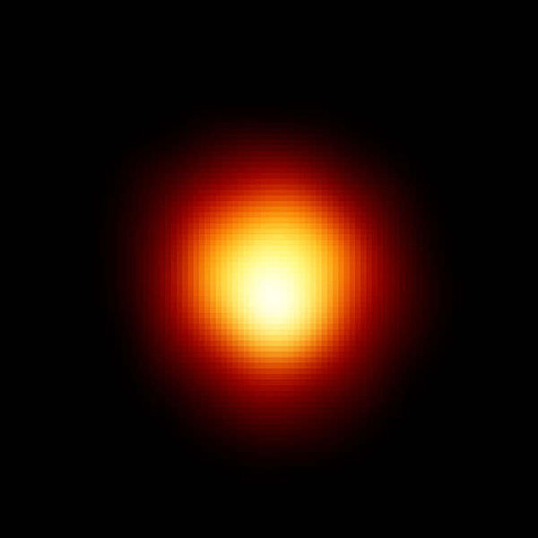
Let’s begin our visual and binocular tour of Orion with its brightest star, Alpha – the “a” symbol on our map. Located in the northeastern corner of Orion and about 425 light years from our solar system, Betelgeuse, like many red giant stars, it is inherently unstable – varying irregularly by as much 1.3 magnitudes in cycles up to six years in length. At its brightest, Betelgeuse can appear more luminous than Rigel (Beta) and its diameter could encompass all the inner planets and much of the asteroid belt. Due to low density, observers would have a hard time determining where space ended and the star began! Allowing for all ranges of radiation, Betelgeuse is more than 50,000 times brighter than our own Sun. Like Antares, it is a “star within a star” – its dense core region radiating with such ferocity that internal pressure drives matter away. Betelgeuse’s core has probably fused all its hydrogen and is now releasing energy through helium fusion – resulting in atoms essential to organic life (carbon and oxygen). Even though it hasn’t gone supernova yet, when it does it will outshine the Moon!

Now, hop to the southwest corner for a look at Beta Orionis – the “B” symbol on our map. Known as Rigel and located about 775 light years from Earth, this hot, blue supergiant star shines with the light of 40,000 suns. If we were to include the amount of light that Rigel produces in the ultra-violet spectrum, too it would produce up to 66,000 times as much light as Sol! But, Rigel also holds a surprise. Point even a small telescope its way and you’ll find out that Beta Orionis is a binary star. Its 7th magnitude companion is separated well away, but you’ll need to keep Rigel to the edge of the field of view to cut the brilliance in order to see it. This small companion orbits about 50 Pluto distances away from its giant companion… which is a good thing since it one day may explode!

Take a look at Gamma Orionis – the “Y” symbol on our map. Bellatrix is known as the “Amazon Star” and is about 240 light years away. While it was once believed to be associated with the other stars of Orion, we’ve learned that Bellatrix is a star in its own right – separate from the others. Historically is was used to measure stellar luminosity until it was discovered that it was an eruptive variable star! While you won’t much notice a tenth of a magnitude change in the 27th brightest star in the sky, it’s still cool to know that it’s collecting a dusty hood that fooled astronomers for many years!

Don’t forget to look at Kappa Orionis, too – the “k” symbol on our map. Even though Saiph is about the same distance away and same size as Rigel, it sure doesn’t look the same, does it? Why? Because Saiph is a much hotter star and most of its light is emitted in the ultraviolet range. It, too, is destined to lead a short, violent stellar life – ending a supernova.

For other interesting stars to take a look at in binoculars, check out U Orionis – it’s a Mira-type variable star. Most of the time U holds an average magnitude of 4.8, Mira-type regular variable is U Orionis, which usually has a brightness of 4.8 but every 368.3 days it drops down to a telescopic magnitude 13! Pi 5 Orionis is a nice visual double star, but even a small telescope and will thoroughly enjoy Sigma Orionis – a true multiple star system. Don’t forget Lambda, too! It’s also a great telescopic binary star!

Because Orion is so loaded with deep sky objects, we’ll only touch on a few of the great for binoculars and telescopes. Absolutely one of the best is Messier 42 located in the asterism of “Orion’s Sword”. Known as the Great Orion Nebula – M42 is actually a great cloud of glowing gases whose size is beyond our comprehension. More than 20,000 times larger than our own solar system, its light is mainly fluorescent. For most people, the Great Orion Nebula will appear to have a slight greenish color – the result of doubly ionized oxygen. At the fueling heart of this immense region is an area known as the Trapezium, its four easily seen stars perhaps the most celebrated multiple system in the night sky. The Trapezium itself belongs to a faint cluster of stars which are now approaching the main sequence stage in an area known as the “Huygenian Region”. Buried in this cloud of mainly hydrogen gas there are many star forming regions amidst the bright ribbons and curls. Appearing like “knots” in the structure, these are known as “Herbig-Haro objectsâ€? and are believed to be stars in their earliest states. There are also a great number of faint reddish stars and erratic variables – very young stars that may be of the accreting T Tauri type. Along with these are “flare starsâ€? whose rapid variations mean that amateur astronomers have a chance to witness new activity. While you view M42, note that the region appears very turbulent. There is a very good reason. The Great Nebula’s many different areas move at different speeds both in recession and approach. The expansion rate at the outer edges of the nebula is an indication of radiation from the very youngest stars known. Although it may be as many as 23,000 years since the Trapezium brought it to “light” it is entirely possible that new stars are still forming in M42. Don’t forget the area of nebulosity that appears slightly separate is designated as M43!

Now, let’s check out the “Running Man” in a large telescope. Located just a half a degree north of M42/43, this tripartite nebula consists of three separate areas of emission and reflection nebulae that seem to be visually connected. NGCs 1977, 1975 and 1973 would probably be pretty spectacular if they were a bit more distant from their grand neighbor! This whispery soft, conjoining nebula’s fueling source is multiple star 42 Orionis. To the eye, a lovely triangle of bright nebulae with several enshrouded stars makes a wonderfully large region for exploration. Can you see the “Running Man” within?

Ready for some open star clusters for your binoculars and telescopes? Hop about four fingerwidths southeast of Betelgeuse for NGC 2186. This large, loose open cluster is well suited to larger binoculars or small telescopes and contains around 50 or so members that range in magnitude from 9 to 11. Look for many distinct pairings! NGC 2186 has been a study area for astronomers and is known to contain circumstellar disks, which may be either newly-forming solar systems or just regenerated materials left over from formation. The next hop is just northwest of apparent double Kappa Orionis. NGC 2194 is also a Herschel object and at magnitude 8.5 is well suited to smaller scopes. This rich galactic cluster can be well resolved in larger scopes and the similar magnitude members make it a delightful spray of stars.

Now, let’s look at some galactic star clusters that belong to different catalogs. The first three are known as “Dolidzes” and your marker star is Gamma Orionis. The first is an easy hop of about one degree northeast of Gamma – Dolidze 21. Here we have what is considered a “poorâ€? open cluster. Not because it isn’t nice – but because it isn’t populous. It is home to around 20 or so low wattage stars of mixed magnitude with no real asterism to make it special. The second is about one degree northwest of Gamma – Dolidze 17. The primary members of this bright group could easily be snatched with even small binoculars and would probably be prettier in that fashion. Five very prominent stars cluster together with some fainter members that are, again, poorly constructed. But it includes a couple of nice visual pairs. Low power is a bonus on this one to make it recognizable. The last is about two degrees north of Gamma – Dolidze 19. Two well-spaced roughly 8th magnitude stars stand right out with a looping chain of far fainter stars between them and a couple of relatively bright members dotted around the edges. With the very faint stars added in, there are probably three dozen stars all told and this one is by far the largest concentration of this “Do” trio.

Now let’s have a look at a deceptive open cluster located in Barnard’s Loop around 2 degrees northeast of bright nebula M78. While billed at a magnitude of roughly 8, NGC 2112 might be a binocular object, but it’s a challenging one. This open cluster consists of around 50 or so stars of mixed magnitudes and only the brightest can be seen in small aperture. Add a little more size in equipment and you’ll find a moderately concentrated, small cloud of stars that is fairly distinguishable against a stellar background. Also known as Collinder 76, this unusual cluster resides in the galactic disc – an area of mostly very old, metal poor stars. It is believed that NGC 2112 is of a more intermediate age, based on recent photometric and spectroscopic data.

Are you ready for a challenge? Then take advantage of dark sky time to head to the eastern-most star in the belt – Zeta Orionis. Alnitak resides at a distance of some 1600 light-years, but this 1.7 magnitude beauty contains many surprises – like being a triple system. Fine optics, high power and steady skies will be needed to reveal its members. About 15′ east and you will see that Alnitak also resides in a fantastic field of nebulosity which is illuminated by our tripartite star. NGC 2024 is an outstanding area of emission that holds a rough magnitude of 8 – viewable in small scopes but requiring a dark sky. So what’s so exciting about a fuzzy patch? Look again, for this beauty is known as the Flame Nebula.

Larger telescopes will deeply appreciate this nebula’s many dark lanes, bright filaments and unique shape. For the large scope, place Zeta out of the field of view to the north at high power and allow your eyes to re-adjust. When you look again, you will see a long, faded ribbon of nebulosity called IC 434 to the south of Zeta that stretches for over a degree. The eastern edge of the “ribbonâ€? is very bright and mists away to the west, but look almost directly in the center for a small dark notch with two faint stars to the south. You have now located one of the most famous of the Barnard dark nebulae – B33. B33 is also known as the Horsehead Nebula. It’s a very tough visual object – the classic chess piece shape is only seen in photographs – but those of you who have large aperture can see a dark “nodeâ€? that is improved with a filter. B33 itself is nothing more than a small area cosmically (about 1 light-year in expanse) of obscuring dark dust, non-luminous gas, and dark matter – but what an incredible shape. If you do not succeed at first attempt? Do not give up. The “Horsehead” is one of the most challenging objects in the sky and has been observed with apertures as small as 150mm.

Now challenge yourself to a 6th magnitude open cluster just northwest of the top star in Orion’s bow (RA 04 49 24 Dec +10 56 00) as we have a look at NGC 1662. Discovered on this night in 1784 and cataloged as H VII.1 by Sir William Herschel, it won’t make the popular lists because it’s nothing more than a double handful of stars…or is it? Studied extensively for proper motion, this galactic cluster may have once held more stars earlier in its lifetime. Enjoy its bright blue and gold members and mark your notes for locating a binocular deep sky object!

Orion is filled with many more great deep sky objects, so get a good star chart and go hunting with the “Hunter”!

Sources:
Wikipedia
Chandra Observatory
Star chart courtesy of Your Sky.

Podcast: Distance in Space, Changing Earth’s Orbit, and Different Sized Stars

Betelgeuse. Image credit: Hubble

[/caption]
This week we find out the distance between Betelgeuse and Bellatrex, how astronomers measure distance between objects, the possibility that an object could mess up the Earth’s orbit, and the reason for different sizes of stars. If you’ve got a question for the Astronomy Cast team, please email it in to [email protected] and we’ll try to tackle it for a future show. Please include your location and a way to pronounce your name.

Click here to download the episode.

Or subscribe to: astronomycast.com/podcast.xml with your podcatching software.

Distance in Space, Changing Earth’s Orbit, and Different Sized Stars – Transcript and show notes.

Astronomers Now Looking For Exomoons Around Exoplanets

An artist impression of an exomoon orbiting an exoplanet, could the exoplanet's wobble help astronomers? (Andy McLatchie)

[/caption]It looks like astronomers have already grown tired of taking direct observations of exoplanets, been there, done that. So they are now pushing for the next great discovery: the detection of exomoons orbiting exoplanets. In a new study, a British astronomer wants to use a technique more commonly associated with the indirect observation of exoplanets. This technique watches a candidate star to see if it wobbles. The wobble is caused by the gravitational pull of the orbiting exoplanet, revealing its presence.

Now, according to David Kipping, the presence of exomoons can also be detected via the “wobble method”. Track an exoplanet during its orbit around a star to see its own wobble due to the gravitational interaction between the exoplanet/exomoon system. As if we needed any more convincing that this is not already an ‘all kinds of awesome’ project, Kipping has another motivation behind watching exoplanets wobble. He wants to find Earth-like exomoons with the potential for extraterrestrial life…

If you sat me in a room and asked me for ten years over and over again: “If you were an astronomer, and you had infinite funds, what would you want to discover?“, I don’t think I would ever arrive at the answer: the natural satellites orbiting exoplanets.” However, now I have read an article about it and studied the abstracts of a few papers, it doesn’t seem like such a strange proposition.

David Kipping, an astronomer working at the University College London (UCL), has acquired funding to investigate his method of measuring the wobble of exoplanets to reveal the presence of exomoons, and to measure their mass and distance from the exoplanet.

Until now astronomers have only looked at the changes in the position of a planet as it orbits its star. This has made it difficult to confirm the presence of a moon as these changes can be caused by other phenomena, such as a smaller planet,” said Kipping. “By adopting this new method and looking at variations in a planet’s position and velocity each time it passes in front of its star, we gain far more reliable information and have the ability to detect an Earth-mass moon around a Neptune-mass gas planet.”

Kipping’s work appeared in the December 11th Monthly Notices of the Royal Astronomical Society and could help the search for exomoons that lie within the habitable zone. Of the 300+ exoplanets observed so far, 30 are within the habitable zones of their host stars, but the planets themselves are large gas giants, several times the size of Jupiter. These gas giants are therefore assumed to be hostile for the formation for life (life as we know it in any case) and so have been discounted as habitable exoplanets.

But what if these exoplanets in the habitable zone have Earth-like exomoons orbiting them? Could they be detected? It would appear so.

Prof. Keith Mason, Chief Executive of the Science and Technology Facilities Council (STFC), added, “It’s very exciting that we can now gather so much information about distant moons as well as distant planets. If some of these gas giants found outside our Solar System have moons, like Jupiter and Saturn, there’s a real possibility that some of them could be Earth-like.”

Watch this space for an announcement of the first Earth-like exomoon to be discovered, at the rate of current technological advancement in astronomy, we could be looking at our first Earth-like exoplanet exomoon sooner than we anticipated…

Source: New Scientist, STFC