Category: Earth Observation

Image credit: NASA

Researchers have discovered that temporary cracks can form in the Earth’s magnetic field that can permit some of the solar wind’s energy to slip through and disrupt electronics and communications. These observations were made using NASA’s Imager for Magnetopause to Aurora Global Exploration (IMAGE) satellite, which tracked a large aurora for several hours. The ESA’s Cluster satellites flew over the same location and spotted a stream of ions slipping through a crack which normally should have been deflected by the Earth’s magnetosphere.

Immense cracks in the Earth’s magnetic field remain open for hours, allowing the solar wind to gush through and power stormy space weather, according to new observations from the IMAGE and Cluster satellites.

The cracks were detected before but researchers now know they can remain open for long periods, rather than opening and closing for just very brief intervals. This new discovery about how the Earth’s magnetic shield is breached is expected to help space physicists give better estimates of the effects of severe space weather.

“We discovered that our magnetic shield is drafty, like a house with a window stuck open during a storm,” said Dr. Harald Frey of the University of California, Berkeley, lead author of a paper on this research published Dec. 4 in Nature. “The house deflects most of the storm, but the couch is ruined. Similarly, our magnetic shield takes the brunt of space storms, but some energy continually slips through its cracks, sometimes enough to cause problems with satellites, radio communication, and power systems.”

“The new knowledge that the cracks are open for long periods, instead of opening and closing sporadically, can be incorporated into our space weather forecasting computer models to more accurately predict how our space weather is influenced by violent events on the Sun,” said Dr. Tai Phan, also of UC Berkeley, co-author of the Nature paper.

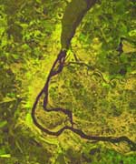
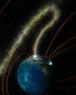
The solar wind is a stream of electrically charged particles (electrons and ions) blown constantly from the Sun (Image 1). The solar wind transfers energy from the Sun to the Earth through the magnetic fields it carries and its high speed (hundreds of miles/kilometers per second). It can get gusty during violent solar events, like Coronal Mass Ejections (CMEs), which can shoot a billion tons of electrified gas into space at millions of miles per hour.

Earth has a magnetic field that extends into space for tens of thousands of miles, surrounding the planet and forming a protective barrier to the particles and snarled magnetic fields the Sun blasts toward it during CMEs. However, space storms, which can dump 1,000 billion watts — more than America’s total electric generating capacity — into the Earth’s magnetic field, indicated that the shield was not impenetrable.

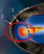
In 1961, Dr. Jim Dungey of the Imperial College, United Kingdom, predicted that cracks might form in the magnetic shield when the solar wind contained a magnetic field that was oriented in the opposite direction to a portion of the Earth’s field. In these regions, the two magnetic fields would interconnect through a process known as “magnetic reconnection,” forming a crack in the shield through which the electrically charged particles of the solar wind could flow. (Image 2 illustrates the crack formation, and Animation 1 shows how solar wind particles flow through the crack by following invisible magnetic field lines.) In 1979, Dr. Goetz Paschmann, of the Max Planck Institute for Extraterrestrial Physics, Germany, detected the cracks using the International Sun Earth Explorer (ISEE) spacecraft. However, since this spacecraft only briefly passed through the cracks during its orbit, it was unknown if the cracks were temporary features or if they were stable for long periods.

In the new observations, the Imager for Magnetopause to Aurora Global Exploration (IMAGE) satellite revealed an area almost the size of California in the arctic upper atmosphere (ionosphere) where a 75-megawatt “proton” aurora flared for hours (Image 4). This aurora, energetic enough to power 75,000 homes, was different from the visible aurora known as the Northern and Southern lights. It was generated by heavy particles (ions) hitting the upper atmosphere and causing it to emit ultraviolet light, which is invisible to the human eye but detectable by the Far Ultraviolet Imager on IMAGE. (Image 6 and Animation 4 show IMAGE’s observations of the proton aurora).

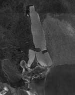
While the aurora was being recorded by IMAGE, the 4-satellite Cluster constellation flew far above IMAGE, directly through the crack, and detected solar wind ions streaming through (Image 5). Normally, these solar wind ions would be deflected by Earth’s shield (Image 3), so Cluster’s observation showed a crack was present. This stream of solar wind ions bombarded our atmosphere in precisely the same region where IMAGE saw the proton aurora. The fact that IMAGE was able to view the proton aurora for more than 9 hours, until IMAGE progressed in its orbit to where it could not observe the aurora, implies that the crack remained continuously open. (Animation 2 shows how the spacecraft worked together to reveal the crack.) Estimating from the IMAGE and Cluster data, the crack was twice the size of the Earth at the boundary of our magnetic shield, about 38,000 miles (60,000 km) above the planet’s surface. Since the magnetic field converges as it enters the Earth in the polar regions, the crack narrowed to about the size of California down near the upper atmosphere.

IMAGE is a NASA satellite launched March 25, 2000 to provide a global view of the space around Earth influenced by the Earth’s magnetic field. The Cluster satellites, built by the European Space Agency and launched July 16, 2000, are making a three-dimensional map of the Earth’s magnetic field.

Original Source: NASA News Release

Image credit: ESA

The Earth’s wetlands are home to some of the most fragile and diverse ecosystems on the planet, and they’re under constant threat from human agriculture, pollution, and settlement. This month the European Space Agency began a program to map 50 wetland areas around the Earth from space to help keep track of their health. ESA’s Envisat is able to tell the difference between dry and waterlogged areas, and will be able to provide annual data about how various wetlands change throughout the seasons.

Dotted across varied regions of our planet are the waterlogged landscapes known as wetlands. Often inaccessible, these muddy areas are actually treasure houses of ecological diversity ? their overall value measured in trillions of Euros.

For much of the last century wetlands have been drained or otherwise degraded, but scientific understanding of their important roles in terms of biology and the water cycle has grown, spurring international efforts to preserve them. On 20 November ESA formally began a project to map wetlands from space, providing data on around 50 sites in 21 countries worldwide.

In 1971 an inter-governmental treaty established the Ramsar Convention on Wetlands, establishing a framework for the stewardship and preservation of wetlands. Today more than 1310 wetlands have been designated as Wetlands of International Importance, a total area of 111 million hectares. The Convention’s 138 national signatories are obliged to report on the state of listed wetlands they are responsible for.

ESA’s new ?1 million Globwetland project is producing satellite-derived and geo-referenced products including inventory maps and digital elevation models of wetlands and the surrounding catchment areas. These products will aid local and national authorities in fulfilling their Ramsar obligations, and should also function as a helpful tool for wetland managers and scientific researchers.

“The Ramsar Convention on Wetlands stresses that targeted assessment and monitoring information is vital for ensuring effective management planning for wetlands, their hydrology and their catchments,” explained Nick Davidson, Ramsar’s Deputy Secretary General. “Yet for wetland managers and decision-makers in many countries access to sound information about wetlands and how they are changing is often a critical gap.

“By working with users at site and catchment scales the Globwetland project should contribute significantly to helping achieve effective management of these critical important ecosystems for biodiversity and human well-being.”

With wetlands often made up of difficult and inaccessible terrain, satellites can help provide information on local topography, the types of wetland vegetation, land cover and use and the dynamics of the local water cycle. In particular radar imagery of the type provided by ESA’s Envisat is able to differentiate between dry and waterlogged surfaces, and so can provide multitemporal data on how given wetlands change seasonally.

Data gathered over four continents
Globwetland products are being provided for a wide range of terrain types to users across four continents: North and South America, Africa, Asia and Europe, including European Russia. In Spain the Globwetland end-user is the government’s Ministry of the Environment.

“We have previously used aerial photography to prepare wetland maps, but this is the first time we will use Earth Observation data,” said Jos? Ram?n Picatoste Ruggeroni, Director General of Nature Conservation and Subdirector General of Biodiversity Conservation. “The areas we are most interested in are land cover and land cover analysis, topography dynamics and subsidence layers, water cycle and quality maps.

“In co-operation with the Spanish regional authorities involved in nature conservation and local wetland managers, we hope to investigate the possibility of achieving a common standard of regularly updated geoinformation to monitor ecological changes in the Spanish Ramsar sites.”

At the other side of the continent, wetlands comprise a third of the territory of the Russian Federation, the majority of it in the form of peatlands. Through much of the 20th century these areas were regarded as wasteland and drained for peat extraction – ending up as unproductive lands that do not contribute either economically or in terms of biodiversity, and also cause ecological problems such as dust storms and uncontrolled carbon dioxide emissions from smouldering peat fires.

In Russia the Globwetland partner is the Ministry of Ecology and Land Use of Moscow region, and has a particular interest in using periodic satellite data to monitor peat fires and estimate how effective a new rewetting project is in preventing further outbreaks.

While in South Africa, Globwetland partner the Department of Environmental Affairs and Tourism (DEAT) seeks to use satellite data to help fulfil its Ramsar obligations for its existing three-site wetlands inventory. The Department also plans to map a separate site, the Prince Edward Islands Special Nature Reserve, for the first time.

South Africa hopes to propose the offshore Reserve for designation as a new Ramsar Wetland of International Importance, but its uncharted nature is currently an obstacle to achieving this. This Southern Ocean site is also being nominated next year as a UNESCO World Heritage Site.

Why are wetlands so valuable?
Studies of wetlands show they store and purify water for domestic use, recharge natural aquifers as they run low, retain nutrients in floodplains, help control flooding and shore erosion and regulate local climate.

Most of all, wetlands support life in spectacular variety and numbers: freshwater wetlands alone are home to four in ten of all the world’s species, and one in eight of global animal species.

An assessment of the monetary value of natural ecosystems published in Nature in 1997 arrived at a figure of 27.7 trillion Euros (33 trillion dollars), with wetland ecosystems making up ?12.5 trillion ($14.9 trillion) ? or 45% – of this total.

Much of human civilisation has been based around river valleys and floodplains. However, global freshwater consumption rose sixfold during the 20th century, a rate more than double that of population growth. And world population is set to rise by 70 million people a year for the next two decades.

Couple that trend with the threat of accelerating climate change, and biologically-productive and hydrologically-stabilising wetlands look like necessities we can ill do without.

Original Source: ESA News Release

Image credit: ESA

The European Space Agency’s Envisat Earth observation satellite captured images of a gigantic iceberg as it broke up during an Antarctic storm. The iceberg, called B-15A, was created in March 2000 when a Jamaican-sized chunk of ice broke away from the Ross Ice Shelf. It broke into smaller pieces shortly after that, but the largest chunk, B-15A grounded itself off the coast and stuck around for a few years. Finally in October, 2003, a giant storm helped split the iceberg up.

ESA’s Envisat satellite was witness to the dramatic last days of what was once the world’s largest iceberg, as a violent Antarctic storm cracked a 160-km-long floe in two.

A series of Envisat Advanced Synthetic Aperture Radar (ASAR) instrument images acquired between mid-September and October record how the bottle-shaped iceberg B-15A was split by the onslaught of powerful storms, waves and ocean currents as its own weight kept it fixed on the floor of Antarctica’s Ross Sea.

ASAR is especially useful for polar operations because its radar signal can pierce thick clouds and works through both day and night. Radar imagery charts surface roughness, so can easily differentiate between different ice types. Old ice ? as on the surface of B-15A ? is rougher than newly formed ice.

B-15A began its existence as B-15 in March 2000 – with an area of 11,655 sq km it was the world’s largest known iceberg. This Jamaica-sized floe was created when it broke away from the Ross Ice Shelf. The initial monster berg split into numerous pieces shortly afterwards, with the largest piece designated B-15A.

Like a wall of ice, B-15A remained a stubborn presence for the next two and a half years, diverting ocean currents. This caused increased ice around Ross Island that disrupted breeding patterns for the local penguin colony and required extra icebreaker activity to maintain shipping access to the US base at McMurdo Sound.

B-15A’s end came in sight on 7 October this year, as 120 kph winds buffeted the grounded iceberg during a storm. Two cracks ran into the heart of the iceberg from opposite ends until finally the entire berg gave way.

The larger of the two new pieces has inherited the name B-15A, and the smaller berg named B-15J. They remain largely locked in place, some 3,800 kilometres south of New Zealand. The bergs could persist there for many years ? a GPS station has been placed on the 3,496 sq km B-15A to enable study of its future progress.

Despite events such as these there is so far no conclusive evidence as to whether polar ice is actually thinning. Next year will see the launch of ESA?s CryoSat mission, a dedicated ice-watching satellite designed to map precise changes in the thickness of polar ice-sheets and floating sea-ice.

CryoSat will be the first satellite to be launched as part of the Agency?s Living Planet Programme. This small research mission will carry a radar altimeter that is based on a heritage from existing instruments, but with several major enhancements to improve the measurement of icy surfaces.

By determining rates of ice-thickness change CryoSat will contribute to our understanding of the relationship between the Earth?s ice cover and global climate.

Original Source: ESA News Release

Image credit: ESA

When a powerful earthquake shook the ground in Alaska a year ago, it also set the Earth’s atmosphere shaking. A team of European scientists used the Global Positioning System to map disturbances in the Earth’s ionosphere after a 7.9 magnitude earthquake struck Denali, Alaska. The ionosphere starts at 75 km and goes up to 1,000 km altitude, and it amplifies any disturbance that happens on the ground beneath it – one millimeter disturbance on the ground could become a 100 metre oscillation at 75 km altitude. This gives scientists a new tool to track earthquakes around the world.

A violent earthquake that cracked highways in Alaska set the sky shaking as well as the land, an ESA-backed study has confirmed.

This fact could help improve earthquake detection techniques in areas lacking seismic networks, including the ocean floor.

A team from the Institut de Physique du Globe de Paris and the California Institute of Technology has successfully used the Global Positioning System (GPS) satellite constellation to map disturbances in the ionosphere following last November?s magnitude 7.9 earthquake in Denali, Alaska.

Their paper has been published in the scientific journal Geophysical Research Letters. The research itself was carried out in support of ESA?s Space Weather Applications Pilot Project, aimed at developing operational monitoring systems for space conditions that can influence life here on Earth.

The ionosphere is an atmospheric region filled with charged particles that blankets the Earth between altitudes of about 75 to 1000 km. It has a notable ability to interfere with radio waves propagating through it.

In the particular case of GPS navigational signals, received on Earth from orbiting satellites, fluctuations in the ionosphere ? known as ‘ionospheric scintillations’ – have the potential to cause signal delays, navigation errors or in extreme cases several hours of service lockouts at particular locations.

But while such interference can be an inconvenience for ordinary GPS users, it represents a boon for scientists. By measuring even much smaller-scale shifts in GPS signal propagation time – caused by variations in local electron density as the signal passes through the ionosphere – researchers have at their fingertips a means of mapping ionospheric fluctuations in near real time.

The French and US team made use of dense networks of hundreds of fixed GPS receivers in place across California. These networks were originally established to measure small ground movements due to geological activity, but they can also be utilised to plot the ionosphere structure across three dimensions and in fine detail.

Then when the Denali earthquake occurred on 3 November 2002, the team had a chance to use this technique to investigate another distinctive property of the ionosphere, its ability to work like a natural amplifier of seismic waves moving across the Earth?s surface.

There are several different types of seismic waves moving the ground during an earthquake, the largest scale and the one that does most of the movement is known as a Rayleigh Wave. This type of wave rolls along the ground up and down and side-to-side, in the same way as a wave rolls along the ocean.

Previous research has established that shock waves from Rayleigh Waves in turn set up large-scale disturbances in the ionosphere. A one millimetre peak-to-peak displacement at ground level can set up oscillations larger than 100 metres at an altitude of 150 km.

What the team were able to do following the Denali quake was detect a distinctive wavefront moving through the ionosphere. “Using the network allowed us to observe the propagation of the waves,” explained co-author Vesna Ducic. “We could also separate the small total electron content signal from the very large total electron content variations related to the daily variation of the ionosphere.”

The team observed a signal two to three times larger than the noise level, arriving about 660 to 670 seconds after the arrival of Rayleigh Waves on the ground. And because around six GPS satellites are visible to every ground receiver they were able to calculate the altitude of maximum perturbation ? around 290 to 300 km up.

The signals were weak and only sampled every 30 seconds, with a maximum resolution of 50 km and the overall noise rate high. But the ionospheric signal observed had a clear pattern consistent with models of seismic behaviour. The hope is that the technique can be improved in future, and used to detect earthquakes in areas without seismic detectors, such as the deep ocean or near islands.

“In the framework of Galileo we plan to develop this research,? said Ducic. “Galileo will double the number of satellites and therefore will allow much more precise maps of the ionosphere. We can also foresee that Europe will develop a dense network of Galileo/GPS stations that will take part in the monitoring of these phenomena.

“ESA, together with the French Ministry of Research and CNES have already decided to fund a pre-operational project called SPECTRE – Service and Products for Ionosphere Electronic Content and Tropospheric Refractive index over Europe from GPS – devoted to the high-resolution mapping of the ionosphere. We will be carrying out mapping above Europe as well as California.

“These investigations will support the French space agency CNES?s DEMETER (Detection of Electro-Magnetic Emissions Transmitted from Earthquake Regions) microsatellite, to be launched in 2004 and devoted to the detection in the ionosphere of seismic, volcanic and man-made signals. These ESA activities will be performed in the framework of the Space Weather Applications Pilot Project.”

The Space Weather Applications Pilot Project is an ESA initiative which has already begun to develop a wide range of application-oriented services based around space weather monitoring.

The co-funded services under development – of which this project is one – also include forecasting disruption to power and communication systems, and the provision of early warning to spacecraft operators of the hazards presented by increased solar and space weather activities. The hope is that an a seismic detection service based on ionospheric measurements may in future supplement existing resources in Europe and elsewhere.

Original Source: ESA News Release

Image credit: ESA

The European Space Agency’s Cluster spacecraft were perfectly positioned to watch the effect of the recent solar storms on the Earth’s magnetosphere. Normally the magnetosphere bubbles out in front of the Earth by about 64,000 km, but during the storm it was down to only 43,000 km. The speed at which the magnetosphere compressed will help scientists calculate the power of the storm, and make more accurate predictions for what will happen in future storms.

On the 24th of October 2003, the SOHO spacecraft registered a huge Coronal Mass Ejection (CME), emitted by the Sun. Several hours later this eruption reached the Earth and was detected by a number of spacecraft including Cluster.

The ACE spacecraft, situated along the Sun/Earth direction, was situated about 1 500 000 km upstream from the Earth, monitoring the solar wind. At about 14:49 UT, ACE recorded a sharp increase on the proton velocity, which jumped from about 450 kms-1 to more than 600 km-1 . The proton density, which was about 3 to 4 particles cm-3 , increased to more than 20. The proton temperature in the solar wind at this instant was also multiplied by a factor of 8.

The four Cluster spacecraft were in the southern magnetospheric lobe, inbound towards their perigee. Note that the Sun, ACE, Cluster and the Earth were almost aligned when the CME was ejected from the Sun. Cluster was situated close to the inner magnetosphere (near to the ring current region) when it detected the effects of the solar wind pressure on the magnetosphere: The sudden increase of the solar wind pressure registered by ACE arrived at the Earth?s magnetosphere about 40 minutes later. It provoked a huge compression of the dayside magnetosphere. The Cluster spacecraft detected this compression by getting suddenly out of the southern magnetospheric lobe into the Magnetosheath. They thus detected the Magnetopause, moving earthward, at about 15:25 UT. They remained into the Magnetosheath until about 17:00 UT, when they were only at a 6.8 RE (Earth radii) distance from the Earth. The transition between the lobes and the Magnetosheath was characterised by an important ion density increase (from close to 0 in the lobe to more than 160 particles cm-3 in the Magnetosheath) as well as a very clear signature in the velocity components, as measured by the CIS experiment onboard Cluster (P.I: Henri R?me).

This is a very unusual position for the Magnetopause, which on the average is standing ahead of the Earth at about 10 to 11 RE. Such compressions can have dramatic space weather effects, particularly to geostationnary satellites which are orbiting the Earth at a distance of about 6.6 RE. Further analysis of the four spacecraft data will tell us at what speed the magnetopause moved which will give information on the strength of the CME.

Original Source: ESA News Release

Image credit: NASA

New images of shrinking sea ice may provide further evidence that the Earth is undergoing significant climate change. NASA scientists compared images of arctic sea ice since 1981 and have measured that it’s shrinking by an average of 9% per decade – summer sea ice in 2002 was a record low levels. The loss of ice could accelerate global warming because liquid water absorbs sunlight instead of reflecting it like ice.

Recently observed change in Arctic temperatures and sea ice cover may be a harbinger of global climate changes to come, according to a recent NASA study. Satellite data — the unique view from space — are allowing researchers to more clearly see Arctic changes and develop an improved understanding of the possible effect on climate worldwide.

The Arctic warming study, appearing in the November 1 issue of the American Meteorological Society’s Journal of Climate, shows that compared to the 1980s, most of the Arctic warmed significantly over the last decade, with the biggest temperature increases occurring over North America.

“The new study is unique in that, previously, similar studies made use of data from very few points scattered in various parts of the Arctic region,” said the study’s author, Dr. Josefino C. Comiso, senior research scientist at NASA’s Goddard Space Flight Center, Greenbelt, Md. “These results show the large spatial variability in the trends that only satellite data can provide.” Comiso used surface temperatures taken from satellites between 1981 and 2001 in his study.

The result has direct connections to NASA-funded studies conducted last year that found perennial, or year-round, sea ice in the Arctic is declining at a rate of nine percent per decade and that in 2002 summer sea ice was at record low levels. Early results indicate this persisted in 2003.

Researchers have suspected loss of Arctic sea ice may be caused by changing atmospheric pressure patterns over the Arctic that move sea ice around, and by warming Arctic temperatures that result from greenhouse gas buildup in the atmosphere.

Warming trends like those found in these studies could greatly affect ocean processes, which, in turn, impact Arctic and global climate, said Michael Steele, senior oceanographer at the University of Washington, Seattle. Liquid water absorbs the Sun’s energy rather than reflecting it into the atmosphere the way ice does. As the oceans warm and ice thins, more solar energy is absorbed by the water, creating positive feedbacks that lead to further melting. Such dynamics can change the temperature of ocean layers, impact ocean circulation and salinity, change marine habitats, and widen shipping lanes, Steele said.

In related NASA-funded research that observes perennial sea-ice trends, Mark C. Serreze, a scientist at the University of Colorado, Boulder, found that in 2002 the extent of Arctic summer sea ice reached the lowest level in the satellite record, suggesting this is part of a trend. “It appears that the summer 2003 — if it does not set a new record — will be very close to the levels of last year,” Serreze said. “In other words, we have not seen a recovery; we really see we are reinforcing that general downward trend.” A paper on this topic is forthcoming.

According to Comiso’s study, when compared to longer term ground-based surface temperature data, the rate of warming in the Arctic over the last 20 years is eight times the rate of warming over the last 100 years.

Comiso’s study also finds temperature trends vary by region and season. While warming is prevalent over most of the Arctic, some areas, such as Greenland, appear to be cooling. Springtimes arrived earlier and were warmer, and warmer autumns lasted longer, the study found. Most importantly, temperatures increased on average by 1.22 degrees Celsius per decade over sea ice during Arctic summer. The summer warming and lengthened melt season appears to be affecting the volume and extent of permanent sea ice. Annual trends, which were not quite as strong, ranged from a warming of 1.06 degrees Celsius over North America to a cooling of .09 degrees Celsius in Greenland.

If the high latitudes warm, and sea ice extent declines, thawing Arctic soils may release significant amounts of carbon dioxide and methane now trapped in permafrost, and slightly warmer ocean water could release frozen natural gases in the sea floor, all of which act as greenhouse gases in the atmosphere, said David Rind, a senior researcher at NASA’s Goddard Institute of Space Studies, New York. “These feedbacks are complex and we are working to understand them,” he added.

The surface temperature records covering from 1981 to 2001 were obtained through thermal infrared data from National Oceanic and Atmospheric Administration satellites. The studies were funded by NASA’s Earth Science Enterprise, which is dedicated to understanding the Earth as an integrated system and applying Earth System Science to improve prediction of climate, weather and natural hazards using the unique vantage point of space.

Original Source: NASA News Release

Image credit: NASA/JPL

New research from NASA shows that glaciers in the Patagonia region of South America are thinning out at an accelerated rate. Researchers compared data from the recent space shuttle topography mission in 2000 against historical surveys from the 1970s and 90s. The Patagonia glaciers are losing mass faster than other icefields, such as those in Alaska, which are five times larger. This different rate of melting is important, because it helps researchers understand some of the factors that could contribute other than just overall global climate change.

The Patagonia Icefields of Chile and Argentina, the largest non-Antarctic ice masses in the Southern Hemisphere, are thinning at an accelerating pace and now account for nearly 10 percent of global sea-level change from mountain glaciers, according to a new study by NASA and Chile’s Centro de Estudios Cientificos.

Researchers Dr. Eric Rignot of NASA’s Jet Propulsion Laboratory, Pasadena, Calif.; Andres Rivera of Universidad de Chile, Santiago, Chile; and Dr. Gino Casassa of Centro de Estudios Cientificos, Valdivia, Chile, compared conventional topographic data from the 1970s and 1990s with data from NASA’s Shuttle Radar Topography Mission, flown in February 2000. Their objective was to measure changes over time in the volumes of the 63 largest glaciers in the region.

Results of the study, published this week in the journal Science, conclude the Patagonia Icefields lost ice at a rate equivalent to a sea level rise of 0.04 millimeters (0.0016 inches) per year during the period 1975 through 2000. This is equal to nine percent of the total annual global sea-level rise from mountain glaciers, according to the 2001 Intergovernmental Panel on Climate Change Scientific Assessment. From 1995 through 2000, however, that rate of ice loss from the icefields more than doubled, to an equivalent sea level rise of 0.1 millimeters (0.004 inches) per year.

In comparison, Alaska’s glaciers, which cover an area five times larger, account for about 30 percent of total annual global sea-level rise from mountain glaciers. So what’s causing the increased Patagonia thinning?

Rignot and his colleagues concluded the answer is climate change, as evidenced by increased air temperatures and decreased precipitation over time. Still, those factors alone are not sufficient to explain the rapid thinning. The rest of the story appears to lie primarily in the unique dynamic response of the region’s glaciers to climate change.

“The Patagonia Icefields are dominated by so-called ‘calving’ glaciers,” Rignot said. “Such glaciers spawn icebergs into the ocean or lakes and have different dynamics from glaciers that end on land and melt at their front ends. Calving glaciers are more sensitive to climate change once pushed out of equilibrium, and make this region the fastest area of glacial retreat on Earth.?

Rignot said the study underscores NASA’s unique contributions to understanding changes in Earth’s cryosphere. “From the unique vantage point of space, the Shuttle Radar Topography Mission provided the first complete topographic coverage of the Patagonia Icefields,” he explained. “Researchers can now access data on this remote Earth region in its totality, allowing them to draw conclusions about the whole system, rather than just focusing on changes on a few glaciers studied from the ground or by aircraft.?

Rignot said scientists are particularly interested in studying how climate interacts with glaciers because it may be a good barometer of how the large ice sheets of Greenland and Antarctica will respond to future climate change. “We know the Antarctic peninsula has been warming for the past four decades, with ice shelves disappearing rapidly and glaciers behind them speeding up and raising sea level,” he noted. “Our Patagonia research is providing unique insights into how these larger ice masses may evolve over time in a warmer climate,” he said.

The Northern Patagonia Icefield in Chile and the Southern Patagonia Icefield in Chile and Argentina, cover 13,000 and 4,200 square kilometers (5,019 and 1,622 square miles), respectively. The region, spanning the Andes mountain range, is sparsely inhabited, with rough terrain and poor weather, restricting ground access by scientists. Precipitation in the region ranges from 2 to 11 meters (6.6 to 36 feet) of water equivalent per year, a snow equivalent of up to 30 meters (98.4 feet) a year. The icefields discharge ice and meltwater to the ocean on the west side and to lakes on the east side, via rapidly flowing glaciers. The fronts of most of these glaciers have been retreating over the past half- century or more.

The study benefited from ground experiments led jointly by Centro de Estudios Cientificos; Universidad de Chile; University of Washington, Seattle; and University of Alaska, Fairbanks, with funding by NASA, Fondecyt (Chilean National Science Foundation) and the National Science Foundation International Program.

The Shuttle Radar Topography Mission is a cooperative project of NASA, the National Imagery and Mapping Agency, and the German and Italian space agencies. Information about the Shuttle Radar Topography Mission is available at: http://www.jpl.nasa.gov/srtm/. The California Institute of Technology in Pasadena manages JPL for NASA.

Original Source: NASA News Release

Image credit: NASA

NASA satellite data has been used to analyze the biology of open area “hotspots” around the coast of Antarctica. The research has found that penguin populations are healthy when there are patches of open water nearby where plankton blooms can form in the sunlight. The plankton feeds shrimp-like krill which supports many other marine animals including penguins. The data was gathered by NASA’s Sea-viewing Wide Field-of-view Sensor (SeaWiFS) and NOAA’s Advanced Very High Resolution Radiometer (AVHRR) which kept weekly records of ocean temperature and plankton levels.

NASA satellite data was used for the first time to analyze the biology of hot spots along the coast of Antarctica. The biological oases are open waters, called polynyas, where blooming plankton support the local food chain.

The research found a strong association between the well being of Adelie Penguin populations in the Antarctic and the productivity of plankton in the polynyas. Polynyas are areas of open water or reduced ice cover, where one might expect sea ice. They are usually created by strong winds that blow ice away from the coast leaving open areas, or by gaps appearing on the ocean’s surface, when flowing ice gets blocked by an impediment, like an ice shelf.

The Antarctic waters are rich in nutrients. The lack of ice, combined with shallow coastal waters, provides the top layers of the ocean with added sunlight, so polynyas offer ideal conditions for phytoplankton blooms. Because the ice around polynyas is thin in the early spring when the long Austral day begins, they are the first areas to get strong sunlight. The open waters retain more heat, further thinning ice cover and leading to early, intense, and short-lived plankton blooms. These blooms feed krill, a tiny, shrimp-like animal, which in turn are eaten by Adelie Penguins, seabirds, seals, whales, and other animals.

Although relatively small in area, coastal polynyas play a disproportionately important role in many physical and biological processes in Polar Regions. In eastern Antarctica, more than 90 percent of all Adelie Penguin colonies live next to coastal polynyas. Polynya productivity explains, to a great extent, the increase and decrease in penguin population.

“It’s the first time anyone has ever looked comprehensively at the biology of the polynyas,” said Kevin Arrigo, assistant professor of Geophysics at Stanford University, Stanford, Calif. “No one had any idea how tightly coupled the penguin populations would be to the productivity of these polynyas. Any changes in production within these polynyas are likely to lead to dramatic changes in the populations of penguins and other large organisms,” Arrigo said.

The study, which appeared in a recent issue of the Journal of Geophysical Research, used satellite-based estimates to look at interannual changes in polynya locations and sizes; abundance of microscopic free-floating marine plants called phytoplankton, which are the base of the polar ocean food chain; and the rate at which phytoplankton populations thrive. Covering five annual cycles from 1997 to 2002, 37 coastal polynya systems were studied.

The largest polynya studied was located in the Ross Sea (396,500 square kilometers or 153,100 square miles; almost the size of California). The smallest was located in the West Lazarev Sea (1,040 square kilometers or 401.5 square miles). Most polynyas, at their maximum area in February, were less than 20,000 square kilometers (7,722 square miles).

Data from NASA’s Sea-viewing Wide Field-of-view Sensor (SeaWiFS) and NOAA’s Advanced Very High Resolution Radiometer (AVHRR) provided weekly measurements of chlorophyll and temperature that were used in a computer model to estimate phytoplankton productivity. The researchers found, taken together, the Ross Sea, Ronne Ice Shelf, Prydz Bay, and Amundsen Sea polynyas were responsible for more than 75 percent of total plankton production.

The researchers were surprised to find how closely connected the Adelie Penguins were to the productivity of their local polynyas. The more productive polynyas supported larger penguin populations. The more abundant krill fed more penguins, and the birds had shorter distances to go to forage, which reduced exposure to predators and other dangers.

The NASA Oceanography Program, the National Science Foundation, and the U.S. Department of Energy funded this research. NASA’s Earth Science Enterprise is dedicated to understanding the Earth as an integrated system and applying Earth System Science to improve prediction of climate, weather, and natural hazards using the unique vantage point of space.

Original Source: NASA News Release

Image credit: NASA

NASA satellites have been watching a gigantic iceberg as it disrupts the fragile Antarctic marine environment. The iceberg, named C-19, is 32 km wide and 200 km long; it broke off the Ross Ice Shelf back in May 2002. The problem is that the iceberg stopped winter sea ice from moving out of the Ross Sea region. Phytoplankton, which needs sunlight, was reduced by 90%, and so the rest of the ecosystem suffered too. The iceberg is being watched with NASA’s Terra and OrbView2 satellites.

NASA satellites observed the calving, or breaking off, of one of the largest icebergs ever recorded, named “C-19.”

C-19 separated from the western face of the Ross Ice Shelf in Antarctica in May 2002, splashed into the Ross Sea, and virtually eliminated a valuable food source for marine life. The event was unusual, because it was the second-largest iceberg to calve in the region in 26 months.

Over the last year, the path of C-19 inhibited the growth of minute, free-floating aquatic plants called phytoplankton during the iceberg’s temporary stopover near Pennell Bank, Antarctica. C-19 is located along the Antarctic coast and has diminished little in size. Since phytoplankton is at the base of the food chain, C-19 affects the food source of higher-level marine plants and animals.

Kevin R. Arrigo and Gert L. van Dijken of Stanford University, Stanford, Calif., used chlorophyll data from NASA’s Sea-viewing Wide Field-of-view Sensor (SeaWiFS). The instrument, on the OrbView-2 satellite, also known as SeaStar, was used to locate and quantify the effects of C-19 on phytoplankton. The researchers were able to pinpoint iceberg positions by using images from the Moderate Resolution Imaging Spectroradiometer (MODIS), an instrument aboard NASA’s Terra and Aqua satellites. The findings from this NASA-funded study appeared in a recent issue of the American Geophysical Union’s Geophysical Research Letters.

C-19 is about twice the size of Rhode Island. When it broke off the Ross Ice Shelf, the iceberg was 32 km (almost 20 miles) wide and 200 km (124 miles) long. It was not as large as the B-15 iceberg that broke off of the same ice shelf in 2001 but among the largest icebergs ever recorded.

Since it was so large, C-19 blocked sea ice from moving out of the southwestern Ross Sea region. The blockage resulted in unusually high sea-ice cover during the spring and summer. Consequently, light was blocked. Phytoplankton blooms that occur on the ocean surface were dramatically diminished, and primary production was reduced by over 90 percent, relative to normal years.

Primary production is the formation of new plant matter by microscopic plants through photosynthesis. Phytoplankton is at the base of the food chain. If they are not able to accomplish photosynthesis, all organisms above them in the food chain will be affected. “Calving events over the last two decades indicate reduced primary productivity may be a typical consequence of large icebergs that drift through the southwestern Ross Sea during spring and summer,” Arrigo said.

Arrigo and van Dijken also used imagery from the Defense Meteorological Satellite Program (DMSP) satellite Special Sensor Microwave Imager and Scanning Multichannel Microwave Radiometer, managed by the U.S. Department of Defense. The data was used to monitor the impact of C-19 on the movement of sea ice. The data is archived at the National Snow and Ice Data Center, University of Colorado, Boulder.

Arrigo said most of the face of the Ross Ice Shelf has already calved. There is another large crack, but it is very difficult to predict if and when another large iceberg will result.

NASA’s Earth Science Enterprise is dedicated to understanding the Earth as an integrated system and applying Earth System Science to improve prediction of climate, weather, and natural hazards using the unique vantage point of space.

Original Source: NASA News Release

Image credit: ESA

The European Space Agency’s demonstrated the capability of its Envisat Earth monitoring satellite to track the water levels of inland lakes and rivers; spots on the Earth that were previously invisible to previous radar altimetry. The Radar Altimeter 2 on board Envisat sends 1800 radar pulses a second from 800 km altitude and then calculates how long they take to return – this tells the device its exact distance to the planet. A team from pored through the raw Envisat data and figured out a way to extract river water levels by spotting specific kinds of radar echos. ESA will release 12 years of river levels for scientists to study.

For over a decade ESA has used satellites to bounce radar pulses off the Earth and precisely measure the height of ocean and land surfaces. But inland lakes and rivers have been effective blind spots for radar altimetry ? at least until now.

Next week ESA previews a new product range called River and Lake Level from Altimetry that provides previously inaccessible information on water levels of major lakes and rivers across the Earth’s surface, derived from Envisat and ERS radar altimeter measurements.

Hydrologists can use this new data to monitor river heights around the planet, assess the impact of global warming and help with water resource management. Inland water bodies are important as key sources of both water and food for the people living round them. They are also often regions of maximum biodiversity and represent early indicators of regional climate change.

A new processing algorithm has been developed to extract rivers and lakes level findings from raw radar altimeter data. The development effort was headed by Professor Philippa Berry of the UK’s De Montfort University: “The new radar altimeter product is a great leap forward for hydrologists. It gives them a new tool to study both the historical changes in water table levels and critically important data to use in forecasting models of water availability, hydroelectric power production, flood and drought events and overall climate changes.”

The Radar Altimeter 2 (RA-2) flown aboard ESA’s Envisat environmental satellite is the improved follow-on to earlier radar altimeters on the ERS-1 and ERS-2 spacecraft. From its 800 km-high polar orbit it sends 1800 separate radar pulses down to Earth per second then records how long their echoes take to return ? timing their journey down to under a nanosecond to calculate the exact distance to the planet below.

Radar altimeters were first flown in space back in the 1970s, aboard NASA’s Skylab and Seasat. These early efforts stayed focused firmly on the oceans, as less-smooth land surfaces returned indecipherable signals. But as the technology improved reliable land height data became available. Envisat’s RA-2 has an innovative ‘four-wheel drive’ tracking system allowing it to maintain radar contract even as the terrain below shifts from ocean to ice or dry land.

But rivers and lakes have proved tougher targets. Large lakes and wide rivers such as the Amazon often returned tantalising ‘wet’ radar signals, but echoes from nearby dry land distorted most such signals.

Believing full-fledged river and lake level monitoring was nevertheless feasible, ESA awarded a contract to De Montfort University to develop a suitable software product, with Lancaster University advising on field hydrology.

The De Montfort University team proceeded by painstakingly combing through many gigabytes of raw data acquired over rivers and lakes, taking note of the type of echo shapes that occurred. They sorted different echo shapes into distinct categories, then created an automated process to recognise these shapes within ‘wet’ signals and eventually extract usable data from them.

“To do this, the shape of each individual echo has to be analysed, and the exact time corresponding to the echo component from the lake or river must be calculated,” explained Professor Berry. “As well as identifying and removing the echo from surrounding land, this process is complicated by the frequent occurrence of islands and sandbars, particularly in river systems. But in the end this approach has been shown to be very effective indeed, with successful retrieval of heights from the majority of the Earth’s major river and lake systems.”

Next week sees the release of the first demonstration products using this new algorithm, containing representative data from the last seven years for rivers and lakes across Africa and South America. The plan is that global altimeter data for the last 12 years will then be reprocessed to provide hydrologists with historical information, invaluable for assessing long-term trends.

ESA also intends to install operational software in its ground segment so eventually the product can be delivered to users in near-real time, within three hours or less of its acquisition from space.

Hydrologists need no previous knowledge of radar altimetry to make use of the new data, with one product known as River Lake Hydrology providing data corresponding to river crossing points, just as though there were actual river gauges in place.

Such gauges are the traditional way that river and lake level measurements are obtained, but their number in-situ has declined sharply in the last two decades. The new product will compensate for this growing lack of ground data.

The other product is called River Lake Altimetry, intended for altimetry specialists, and provides all crossing points for a water body, together with detailed information on all instrumental and geophysical corrections.

Previews of both products can be accessed via a dedicated website (see right hand bar) or on a free CD ? email [email protected] to order a copy. Both products are being formally announced at the Hydrology from Space conference, beginning Monday 29 September in Toulouse.

Original Source: ESA news release