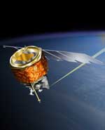
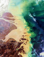
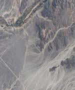
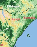
NASA Announces Two New Earth Observation Satellite Missions

Image credit: NASA/Hampton University
Two NASA missions to explore the boundaries of Earth’s atmosphere with space are scheduled for launch in 2006. Both have recently completed preliminary design phases and are ready to proceed with hardware fabrication, integration and testing.

The Aeronomy of Ice in the Mesosphere (AIM) Small Explorer will determine the causes of Earth’s highest-altitude clouds, which occur on the very edge of space. These clouds form in the coldest part of the atmosphere, about 50 miles above the polar-regions, every summer. Recorded sightings of these silvery-blue, noctilucent or “night-shining” clouds began in the late 1800’s at high latitudes. They have been increasing in frequency and extending to lower latitudes over the past four decades.

Scientists have hypothesized the more frequent occurrences may be an indicator of global warming, but until now they have not been able to test this idea. Since similar thin high altitude clouds have been observed at Mars, what AIM teaches us about Earth’s noctilucent clouds should help us understand the similarities and differences between the martian and terrestrial atmospheres.

AIM will measure all the parameters important to understanding noctilucent cloud formation. This will help determine the connection between the clouds and their environment and serve as a baseline for the study of long-term changes in the upper atmosphere. Dr. James Russell III of Hampton University in Hampton, Va., leads AIM as Principal Investigator.

The second mission is the Time History of Events and Macroscale Interactions during Substorms mission (THEMIS). A Medium Explorer mission, it will fly five small spacecraft through explosive geomagnetic disturbances to solve the mystery of what triggers the colorful eruptions of the Northern and Southern lights. These violent “substorms” reflect major reconfigurations of near-Earth space and have significant implications for space weather, affecting satellites and terrestrial communications.

Over the years several different hypotheses have been proposed to explain this phenomenon. THEMIS will use five probes, strategically placed in different regions of the magnetosphere, to determine which explanation is correct. THEMIS is led by Dr. Vassilis Angelopoulos of the University of California, Berkeley.

The Explorer Program is designed to provide frequent, low-cost access to space for physics and astronomy missions with small to mid-sized spacecraft. NASA’s Goddard Space Flight Center, Greenbelt, Md., manages the Explorer Program for the Office of Space Science, Washington.

For information and artists’ concepts of the AIM mission on the Internet, visit:
http://aim.hamptonu.edu/

For Information and artists’ concepts of the THEMIS mission, visit:
http://sprg.ssl.berkeley.edu/themis/

For information about the Explorer program on the Internet, visit:
NASA News Release

For information about NASA and agency missions on the Internet, visit:
http://www.nasa.gov

Original Source: NASA News Release

Arctic Ice Formation is More Complex Than Previously Thought

Image credit: NASA/JPL
Contrary to historical observations, sea ice in the high Arctic undergoes very small, back and forth movements twice a day, even in the dead of winter. It was once believed ice deformation at such a scale was almost non-existent.

According to a recent NASA-funded study, the finding is significant. Such movements may substantially increase the production of new ice and should be factored into Arctic climate models. The phenomenon of short-period Arctic sea ice motion was investigated in detail in 1967 and has been the subject of numerous research studies since.

A 1978 study found short-period ice motions disappeared almost entirely during the winter once the Arctic Ocean froze. A subsequent investigation in 2002, conducted using measurements from ocean buoys spaced hundreds of kilometers apart, found sea ice movement occurs during all seasons.

Since buoy observations are poor for understanding short-length-scale motion and deformation, researchers Ron Kwok and Glenn Cunningham of NASA’s Jet Propulsion Laboratory, Pasadena, Calif., and William Hibler III of the University of Alaska, Fairbanks, set out to examine the phenomenon in greater detail.

The researchers used high-resolution synthetic aperture radar imagery from Canada’s RADARSAT Earth observation satellite, which can image the region up to five times a day. Their findings were published recently in Geophysical Research Letters. The researchers studied an approximate 200 by 200 kilometer (124 by 124 mile) area in the Canada Basin region of the high Arctic for about three weeks in May 2002 and in February 2003.

This region is representative of the behavior of the central Arctic Ocean ice cover due to its location and thickness. The time frame was selected because Arctic sea ice motion is least expected during those times of year.

The study provided a more detailed picture of the phenomenon reported in the 2002 buoy research. It found sea ice moved back and forth and deformed slightly in a persistent 12-hour oscillating pattern. Subtle motions triggered by the Earth’s rotation rather than by tidal movement likely caused the pattern. In the absence of external forces, any object will move in a circular motion due to the Earth’s rotation. The researchers attributed the winter behavior of the ice cover, not observed in studies before 1970, to either a previous lack of detailed data or perhaps an indication of recent thinning of the Arctic ice cover.

“If Arctic pack ice is continually opening and closing during the Arctic winter on a widespread basis, it could significantly increase the rate of Arctic ice production and therefore increase the total amount of ice in the Arctic,” Kwok said. “A simple simulation of this ice production process shows that it can account for an equivalent of 10 centimeters (4 inches) of ice thickness over 6 months of winter. That’s approximately 20 percent of the base growth of thick ice during the central Arctic winter.”

Kwok said current models of the dynamics of Arctic sea ice typically don’t take into account processes occurring at short, 12-hour time scales, and the impact of such processes must be assessed. “As climate models continue to get better and better, it becomes increasingly important to understand the physics of small-scale processes so that we can understand their large-scale consequences,” he said. “If these Arctic sea ice processes are indeed important over the entire Arctic basin, their contribution to the overall amount of ice in the Arctic should be included in simulations of the interactions that take place between the Arctic’s ice, ocean and atmosphere to create the overall Arctic climate.

“If such oscillations in Arctic sea ice increase as the sea ice cover thins due to warmer atmospheric temperatures, then this mechanism of ice production may actually serve to slow down the overall depletion of ice in the Arctic Ocean,” he added. Kwok said other parts of the Arctic Ocean would be analyzed in future studies.

For more information about the study on the Internet, visit http://www.earth.nasa.gov/flash_top.html.

For information about NASA on the Internet, visit http://www.nasa.gov/home/index.html.

JPL is managed for NASA by the California Institute of Technology in Pasadena.

Original Source: NASA/JPL News Release

Satellites Show How the Earth is Warming Up

Image credit: NASA
Like thermometers in space, satellites are taking the temperature of the Earth’s surface or skin. According to scientists, the satellite data confirm the Earth has had an increasing “fever” for decades.

For the first time, satellites have been used to develop an 18- year record (1981-1998) of global land surface temperatures. The record provides additional proof that Earth’s snow-free land surfaces have, on average, warmed during this time period, according to a NASA study appearing in the March issue of the Bulletin of the American Meteorological Society. The satellite record is more detailed and comprehensive than previously available ground measurements. The satellite data will be necessary to improve climate analyses and computer modeling.

Menglin Jin, the lead author, is a visiting scientist at NASA’s Goddard Space Flight Center, Greenbelt, Md., and a researcher with the University of Maryland, College Park, Md. Jin commented until now global land surface temperatures used in climate change studies were derived from thousands of on-the- ground World Meteorological Organization (WMO) stations located around the world, a relatively sparse set of readings given Earth’s size. These stations actually measure surface air temperature at two to three meters above land, instead of skin temperatures. The satellite skin temperature dataset is a good complement to the traditional ways of measuring temperatures.

A long-term skin temperature data set will be essential to illustrate global as well as regional climate variations. Together with other satellite measurements, such as land cover, cloud, precipitation, and sea surface temperature measurements, researchers can further study the mechanisms responsible for land surface warming.

Furthermore, satellite skin temperatures have global coverage at high resolutions, and are not limited by political boundaries. The study uses Advanced Very High Resolution Radiometer Land Pathfinder data, jointly created by NASA and the National Oceanic and Atmospheric Administration (NOAA) through NASA’s Earth Observing System Program Office. It also uses recently available NASA Moderate Resolution Imaging Spectroradiometer skin temperature measurements, as well as NOAA TIROS Operational Vertical Sounder (TOVS) data for validation purposes. All these data are archived at NASA’s Distributed Active Archive Center.

Inter-annually, the 18-year Pathfinder data in this study showed global average temperature increases of 0.43 Celsius (C) (0.77 Fahrenheit (F)) per decade. By comparison, ground station data (2 meter surface air temperatures) showed a rise of 0.34 C (0.61 F) per decade, and a National Center for Environmental Prediction reanalysis of land surface skin temperature showed a similar trend of increasing temperatures, in this case 0.28 C (0.5 F) per decade. Skin temperatures from TOVS also prove an increasing trend in global land surface temperatures. Regional trends show more temperature variations.

“Although an increasing trend has been observed from the global average, the regional changes can be very different,” Jin said. “While many regions were warming, central continental regions in North America and Asia were actually cooling.”

One issue with the dataset is that it cannot detect surface temperatures over snow. In winter, most of the land areas in the mid to upper latitudes of the Northern Hemisphere are covered by snow. Of Earth’s land area, 90 percent of it is snow free in July, compared to only 65 percent in January. For this reason, the study only focused on snow free areas. Still, in mountainous areas that are hard to monitor, like Tibet, satellites can detect the extent of snow coverage and its variations.

The satellite dataset allows researchers to also look at daily trends on global and regional scales. The largest daily variation was above 35.0 C (63 F) at tropical and sub-tropical desert areas for a July 1988 sample, with decreasing daily ranges towards the poles, in general. Daily changes were also closely related to vegetation cover. The daily skin temperature range showed a decreasing global mean trend over the 18-year period, resulting from greater temperature increases at night compared to daytime.

Things like clouds, volcanic eruptions, and other factors gave false readings of land temperatures, but scientists factored those out to make the skin temperature data more accurate. Scientists are considering extending this 18-year satellite- derived skin temperature record up to 2003. The mission of NASA’s Earth Science Enterprise is to develop a scientific understanding of the Earth system and its response to natural or human-induced changes to enable improved prediction capability for climate, weather, and natural hazards. NASA funded the study.

Original Source: NASA News Release

Field Reversal Takes 7,000 Years

Image credit: NASA
The time it takes for Earth’s magnetic field to reverse polarity is approximately 7000 years, but the time it takes for the reversal to occur is shorter at low latitudes than at high latitudes, a geologist funded by the National Science Foundation (NSF) has concluded. Brad Clement of Florida International University published his findings in this week’s issue of the journal Nature. The results are a major step forward in scientists’ understanding of how Earth?s magnetic field works.

The magnetic field has exhibited a frequent but dramatic variation at irregular times in the geologic past: it has completely changed direction. A compass needle, if one existed then, would have pointed not to the north geographic pole, but instead to the opposite direction. Such polarity reversals provide important clues to the nature of the processes that generate the magnetic field, said Clement.

Since the time of Albert Einstein, researchers have tried to nail down a firm time-frame during which reversals of Earth’s magnetic field occur. Indeed, Einstein once wrote that one of the most important unsolved problems in physics centered around Earth’s magnetic field. Our planet’s magnetic field varies with time, indicating it is not a static or fixed feature. Instead, some active process works to maintain the field. That process is most likely a kind of dynamic action in which the flowing and convecting liquid iron in Earth’s outer core generates the magnetic field, geologists believe.

Figuring out what happens as the field reverses polarity is difficult because reversals are rapid events, at least on geologic time scales. Finding sediments or lavas that record the field in the act of reversing is a challenge. In the past several years, however, new polarity transition records have been acquired in sediment cores obtained through the international Ocean Drilling Program, funded by NSF. These records make it possible to determine the major features of reversals, Clement said.

“It is generally accepted that during a reversal, the geomagnetic field decreases to about 10 percent of its full polarity value,” said Clement. “After the field has weakened, the directions undergo a nearly 180 degree change, and then the field strengthens in the opposite polarity direction. A major uncertainty, however, has remained regarding how long this process takes. Although this is usually the first question people ask about reversals, scientists have been forced to answer with only a vague ‘a few thousand years.'”

The reason for this uncertainty? Each published polarity transition reported a slightly different duration, from just under 1,000 years to 28,000 years.

“Now, through the innovative use of deep-ocean sediment cores, Clement has demonstrated that magnetic field reversal events occur within certain time-frames, regardless of the polarity of the reversal,” said Carolyn Ruppel, program director in NSF’s division of ocean sciences. “Sediment cores originally drilled to meet disparate scientific objectives have led to a result of global significance, which underscores the value of collecting and maintaining cores and associated data.”

Clement examined the database of existing polarity transition records of the past four reversals. The overall average duration, he found, is 7,000 years. But the variation is not random, he said. Instead it alters with latitude. The directional change takes half as long at low-latitude sites as it does at mid- to high-latitude sites. “This dependence of duration on site latitude was surprising at first, but it?s exactly as would be predicted in geometric models of reversing fields,” Clement said.

Original Source: NSF News Release

Yangtze River From Space

Image credit: ESA
The coloured waters shown here in this 21 March Envisat Medium Resolution Imaging Spectrometer (MERIS) image have concluded a long journey across China.

They are surging into the East China Sea from the mouth of the Yangtze River, which at 6300 km long is the longest river in Asia and the third longest in the world.

Rising in the Qinghai-Tibetan Plateau, the Yangtze River snakes through nine provinces and serves as a drain for 1.8 million square kilometres of territory. MERIS is designed to detect ocean colour, and clearly visible here is how the Yangtze’s heavy sediment plume discharges into and colours the waters along the Chinese coast. Its total sediment load is estimated at 680 million tonnes a year ? equivalent in weight to a hundred Great Pyramids.

Shanghai – China’s largest city – is located south of the Yangtze mouth and the 1000-km-long navigable stretch of the Yangtze west of it is a zone of major economic activity. The downside of recent growth has been a decrease in water quality that the Chinese government say it intends to combat. At the start of the month an accidental chemical spill into a tributary of the Yangtze temporarily deprived almost a million people of drinking water.

Original Source: ESA News Release

New Research Helps Explain Dust Bowl Drought

Image credit: NOAA
NASA scientists have an explanation for one of the worst climatic events in the history of the United States, the “Dust Bowl” drought, which devastated the Great Plains and all but dried up an already depressed American economy in the 1930’s.

Siegfried Schubert of NASA’s Goddard Space Flight Center, Greenbelt, Md., and colleagues used a computer model developed with modern-era satellite data to look at the climate over the past 100 years. The study found cooler than normal tropical Pacific Ocean surface temperatures combined with warmer tropical Atlantic Ocean temperatures to create conditions in the atmosphere that turned America’s breadbasket into a dust bowl from 1931 to 1939. The team’s data is in this week’s Science magazine.

These changes in sea surface temperatures created shifts in the large-scale weather patterns and low level winds that reduced the normal supply of moisture from the Gulf of Mexico and inhibited rainfall throughout the Great Plains.

“The 1930s drought was the major climatic event in the nation’s history,” Schubert said. “Just beginning to understand what occurred is really critical to understanding future droughts and the links to global climate change issues we’re experiencing today,” he said.

By discovering the causes behind U.S. droughts, especially severe episodes like the Plains’ dry spell, scientists may recognize and possibly foresee future patterns that could create similar conditions. For example, La Ni?as are marked by cooler than normal tropical Pacific Ocean surface water temperatures, which impact weather globally, and also create dry conditions over the Great Plains.

The researchers used NASA’s Seasonal-to-Interannual Prediction Project (NSIPP) atmospheric general circulation model and agency computational facilities to conduct the research. The NSIPP model was developed using NASA satellite observations, including; Clouds and the Earth’s Radiant Energy System radiation measurements; and the Global Precipitation Climatology Project precipitation data.

The model showed cooler than normal tropical Pacific Ocean temperatures and warmer than normal tropical Atlantic Ocean temperatures contributed to a weakened low-level jet stream and changed its course. The jet stream, a ribbon of fast moving air near the Earth’s surface, normally flows westward over the Gulf of Mexico and then turns northward pulling up moisture and dumping rain onto the Great Plains. As the low level jet stream weakened, it traveled farther south than normal. The Great Plains dried up and dust storms formed.

The research shed light on how tropical sea surface temperatures can have a remote response and control over weather and climate. It also confirmed droughts can become localized based on soil moisture levels, especially during summer. When rain is scarce and soil dries, there is less evaporation, which leads to even less precipitation, creating a feedback process that reinforces lack of rainfall.

The study also shed light on droughts throughout the 20th century. Analysis of other major U.S. droughts of the 1900s suggests a cool tropical Pacific was a common factor. Schubert said simulating major events like the 1930s drought provides an excellent test for computer models. While the study finds no indication of a similar Great Plains drought in the near future, it is vital to continue studies relating to climate change. NASA’s current and planned suite of satellite sensors is uniquely poised to answer related climate questions.

Original Source: NASA News Release

Tracking Diseases from Space

Image credit: NASA
Last year more than a million people died of malaria, mostly in Sub-saharan Africa. Outbreaks of Dengue Fever, hantavirus, West Nile Fever, Rift Valley Fever, and even Plague still occasionally strike villages, towns, and whole regions. To the dozens or hundreds who suffer painful deaths, and to their loved ones, these diseases must seem to spring upon them from nowhere.

Yet these diseases are not without rhyme or reason. When an outbreak occurs, often it is because environmental conditions such as rainfall, temperatures, and vegetation set the stage for a population surge in disease-carrying pests. Mosquitoes or mice or ticks thrive, and the diseases they carry spread rapidly.

So why not watch these environmental factors and warn when conditions are ripe for an outbreak? Scientists have been tantalized by this possibility ever since the idea was first expressed by the Russian epidemiologist E. N. Pavlovsky in the 1960s. Now technology and scientific know-how are catching up with the idea, and a region-wide early warning system for disease outbreaks appears to be within reach.

Ronald Welch of NASA’s Global Hydrology and Climate Center in Huntsville, Alabama, is one of the scientists working to develop such an early warning system. “I have been to malarious areas in both Guatemala and India,” he says. “Usually I am struck by the poverty in these areas, at a level rarely seen in the United States. The people are warm and friendly, and they are appreciative, knowing that we are there to help. It feels very good to know that you are contributing to the relief of sickness and preventing death, especially the children.”

The approach employed by Welch and others combines data from high-tech environmental satellites with old-fashioned, “khaki shorts and dusty boots” fieldwork. Scientists actually seek out and visit places with disease outbreaks. Then they scrutinize satellite images to learn how disease-friendly conditions look from space. The satellites can then watch for those conditions over an entire region, country, or even continent as they silently slide across the sky once a day, every day.

In India, for example, where Welch is doing research, health officials are talking about setting up a satellite-based malaria early warning system for the whole country. In coordination with mathematician Jia Li of the University of Alabama at Huntsville and India’s Malaria Research Center, Welch is hoping to do a pilot study in Mewat, a predominantly rural area of India south of New Delhi. The area is home to more than 700,000 people living in 491 villages and 5 towns, yet is only about two-thirds the size of Rhode Island.

“We expect to be able to give warnings of high disease risk for a given village or area up to a month in advance,” Welch says. “These ‘red flags’ will let health officials focus their vaccination programs, mosquito spraying, and other disease-fighting efforts in the areas that need them most, perhaps preventing an outbreak before it happens.”

Outbreaks are caused by a bewildering variety of factors.

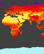
For the mosquito species that carries malaria in Welch’s study area, for example, an outbreak hotspot would have pools of stagnant water where adult mosquitoes can deposit their eggs to mature into new adults. These could be lingering puddles on dense, clay-like soil after heavy rains, swamplands located nearby, or even rain-filled buckets habitually left outside by villagers. A malaria hotspot would be warmer than 18?C, because in colder weather, the single-celled “plasmodium” parasite that actually causes malaria operates too slowly to go through its infection cycle before the host mosquito dies. But the weather mustn’t be too hot, or the mosquitoes would have to hide in the shade. The humidity must hover in the 55% to 75% range that these mosquitoes require for survival. Preferably there would be cattle or other livestock within the mosquitoes’ 1 km flight range, because these pests actually prefer to feed on the blood of animals.

If all of these conditions coincide, watch out!

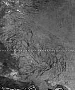
Documenting some of these factors, such as soil type and local bucket-leaving habits, requires initial groundwork by researchers in the field, Welch notes. This information is plugged into a computerized mapping system called a Geographical Information Systems database (GIS). Fieldwork is also required to characterize how the local species of mosquito behaves. Does it bite people indoors or outdoors or both? Other factors, like the locations of cattle pastures and human dwellings, are inputted into the GIS map based on ultra-high resolution satellite images from commercial satellites like Ikonos and QuickBird, which can spot objects on the ground as small as 80 cm across. Then region-wide variables like temperature, rainfall, vegetation types, and soil moisture are derived from medium-resolution satellite data, such as from Landsat 7 or the MODIS sensor on NASA’s Terra satellite. (MODIS stands for MODerate-resolution Imaging Spectrometer.)

Scientists feed all of this information into a computer simulation that runs on top of a digital map of the landscape. Sophisticated mathematical algorithms chew on all these factors and spit out an estimate of outbreak risk.

The basic soundness of this approach for estimating disease risk has been borne out by previous studies. A group from the University of Nevada and the Desert Research Institute were able to “predict” historical rates of deer-mouse infection by the Sin Nombre virus with up to 80% accuracy, based only on vegetation type and density, elevation and slope of the land, and hydrologic features, all derived from satellite data and GIS maps. A joint NASA Ames / University of California at Davis study achieved a 90% success rate in identifying which rice fields in central California would breed large numbers of mosquitoes and which would breed fewer, based on Landsat data. Another Ames project predicted 79% of the high-mosquito villages in the Chiapas region of Mexico based on landscape features seen in satellite images.

Perfect predictions will likely never be possible. Like weather, the phenomenon of human disease is too complicated. But these encouraging results suggest that reasonably accurate risk estimates can be achieved by combining old-fashioned fieldwork with the newest in satellite technologies.

“All of the necessary pieces of the puzzle are there,” Welch says, offering the hope that soon disease outbreaks that seem to come “from out of nowhere” will catch people off guard much less often.

Original Source: NASA Science Story

Santa Ana Winds Stimulate Marine Environment

Image credit: NASA/JPL
Southern California’s legendary Santa Ana winds wreak havoc every year, creating hot, dry conditions and fire hazards. Despite their often-destructive nature, a study of the “Devil Winds,” conducted using data from NASA’s Quick Scatterometer (Quikscat) spacecraft and its SeaWinds instrument shows the winds have some positive benefits.

“These strong winds, which blow from the land out into the ocean, cause cold water to rise from the bottom of the ocean to the top, bringing with it many nutrients that ultimately benefit local fisheries,” said Dr. Timothy Liu, a senior research scientist at NASA’s Jet Propulsion Laboratory, Pasadena, Calif., and Quikscat project scientist. Santa Ana consequences include vortices of cold water and high concentrations of chlorophyll 400 to 1,000 kilometers (248 to 621 miles) offshore.

Liu and Dr. Hua Hu of the California Institute of Technology, Pasadena, in a paper published last year in Geophysical Research Letters, revealed satellite observations of the Santa Ana effects on the ocean during three windy days in February 2003. According to the findings, Quikscat was able to identify the fine features of the coastal Santa Ana wind jets. It identified location, strength and extent, which other weather prediction products lack the resolution to consistently show, and moored ocean buoys lack sufficient coverage to fully represent.

Quikscat’s high-resolution images of air-sea interaction were used to measure wind forces on the ocean. Other satellites and instruments, like the Sea-viewing Wide Field-of-view Sensor (SeaWiFS) and the Advanced Very High Resolution Radiometer, onboard a National Oceanic and Atmospheric Administration polar orbiting weather satellite, were used to measure the temperature and biological production of the ocean surface, which respond to the wind.

The latter instrument showed sea surface temperatures dropped four degrees Celsius (seven degrees Fahrenheit) during the February 2003 Santa Anas. That was a sign that upwelling had occurred, meaning, deep cold water moved up to the ocean surface bringing nutrients. Images from SeaWiFS confirmed the increased biological productivity by measuring chlorophyll concentrations in the surface water. It went from negligible, in the absence of winds, to very active biological activity (more than 1.5 milligrams per cubic meter) in the presence of the winds.

“There really is no other system that can monitor Santa Ana winds over the entire oceanic region,” Liu said. “Scatterometers such as Quikscat have a large enough field of view and high enough resolution to easily identify the details of coastal winds, which can affect the transportation, ecology and economy of Southern California.”

High pressure develops inland when cold air is trapped over the mountains, driving the dry, hot and dusty Santa Anas (also called Santanas and Devil’s Breath) at high speeds toward the coast. The winds, occurring in fall, winter and spring, can reach 113 kilometers (70 miles) per hour. They happen at any time of day and usually reach peak strength in December. Telltale signs on the coast include good visibility inland, unusually low humidity and an approaching dark brown dust cloud.

The Quikscat satellite, launched in June 1999, operates in a Sun- synchronous, 800-kilometer (497-mile) near-polar orbit. It circles Earth every 100 minutes and takes approximately 400,000 daily measurements over 93 percent of the planet’s surface. It passes over Southern California about twice a day, skipping a day every three or four days.

Quikscat is part of an integrated Earth observation system managed by NASA’s Office of Earth Science. The NASA enterprise is dedicated to understanding the Earth as an integrated system and applying Earth System Science to improve prediction of climate, weather, and natural hazards using the unique vantage point of space.

For information about NASA programs on the Internet, visit:

http://www.nasa.gov.

For information about Quikscat and SeaWinds on the Internet, visit:

http://winds.jpl.nasa.gov.

Original Source: NASA/JPL News Release

NASA Finds Smoke Can Choke Clouds

Image credit: NASA
Using data from NASA’s Aqua satellite, agency scientists found heavy smoke from burning vegetation inhibits cloud formation. The research suggests the cooling of global climate by pollutant particles, called “aerosols,” may be smaller than previously estimated.

During the August-October 2002 burning season in South America’s Amazon River basin, scientists observed cloud cover decreased from about 40 percent in clean-air conditions to zero in smoky air.

Until recently, scientists thought aerosols such as smoke particles mainly served to cool the planet by shading the surface, either directly, by reflecting sunlight back toward space, or indirectly, by making clouds more reflective. Certain aerosols make clouds’ droplets smaller and more numerous, thereby making the clouds more reflective while reducing the amount of sunlight reaching the surface.

However, this new study proves smoke aerosols have a “semi- direct” effect on climate, causing a reduction in cloud cover and warming the surface. In the morning, smoke absorbs incoming solar radiation and heats the atmosphere while cooling the surface. Since there is less upward transport of warmth and moisture in such conditions, clouds are less likely to form. Then, in the afternoon, since there is less cloud cover, more sunlight passes through the atmosphere and warms the surface.

“This instantaneous warming is important and can dramatically affect the people and the Amazonian ecosystem,” said Ilan Koren, research scientist at NASA’s Goddard Space Flight Center in Greenbelt, Md.

Koren is lead author of a paper in the current issue of Science. Using Aqua data, Koren and his NASA co-authors measured the total amount of light reflected through the top of the atmosphere. From those data they determined how much area was covered by clouds and how much by smoke. They also estimated the smoke’s “optical thickness,” a measure of how much sunlight the smoke prevented from traveling down through a column of atmosphere.

The team found the smoke and clouds together would ordinarily reflect solar energy equal to one 28-watt light bulb per square meter back up into space (i.e., a cooling effect). With the reduction in cloud cover, however, solar energy equal to one eight-watt light bulb per square meter is absorbed within Earth’s climate system (i.e., a warming effect).

The team consulted other weather data to make sure the differences in cloud patterns were not due to regional differences in meteorology. Once team members proved the meteorological conditions were the same in the smoky regions as they were in the cloudy regions, they knew the smoke had to be the reason average cloud cover dropped from 40 percent to zero in the presence of heavy smoke.

“We used to think of smoke mainly as a reflector, reflecting sunlight back to space, but here we show that, due to absorption, it chokes off cloud formation,” Koren said.

According to Koren, smoke inhibition of cloud formation is not unique to the Amazon area. His team has seen similar examples in other parts of the world, including over parts of Africa during the burning season, and over Canada during major boreal forest wildfires. When added up over the entire globe, the warming influence of smoke and other absorbing aerosols suggests the global cooling influence of these particles is much smaller than current models predict.

Smoke and aerosol inhibition of cloud formation was first proposed in two previous NASA studies based upon results of computer model experiments. However, this study documents the first time this effect of smoke on clouds has been measured in Earth’s environment. The research was funded by NASA’s Earth Science Enterprise. The Enterprise is dedicated to understanding the Earth as an integrated system and applying Earth system science to improve predication of climate, weather and natural hazards using the unique vantage point of space.

Original Source: NASA News Release

Nasca Lines Imaged from Orbit

Image credit: ESA
Visible from ESA’s Proba spacecraft 600 kilometres away in space are the largest of the many Nasca Lines; ancient desert markings now at risk from human encroachment as well as flood events feared to be increasing in frequency.

Designated a World Heritage Site in 1994, the Lines are a mixture of animal figures and long straight lines etched across an area of about 70 km by 30 km on the Nasca plain, between the Andes and Pacific Coast at the southern end of Peru. The oldest lines date from around 400 BC and went on being created for perhaps a thousand years.

They were made simply enough, by moving dark surface stones to expose pale sand beneath. However their intended purpose remains a mystery. It has variously been proposed they were created as pathways for religious processions and ceremonies, an astronomical observatory or a guide to underground water resources.

The Nasca Lines have been preserved down the centuries by extreme local dryness and a lack of erosion mechanisms, but are now coming increasingly under threat: it is estimated the last 30 years saw greater erosion and degradation of the site than the previous thousand years before them.

In this image, acquired by the Compact High Resolution Imaging Spectrometer (CHRIS) instrument aboard Proba on 26 September 2003, the 18.6 metre resolution is too low to make out the animal figures although the straight Nasca Lines can be seen faintly. Clearest of the straight markings is actually the Pan-American Highway, built right through the region ? seen as a dark marking starting at the irrigated fields beside the Ingenio River, running from near the image top to the bottom right hand corner. Associated dirt track roads are also visible amidst the Nasca Lines.

Clearly shown in the Proba image is another cause of damage to the Lines: deposits left by mudslides after heavy rains in the Andean Mountains. These events are believed to be connected to the El Ni?o phenomenon in the Pacific Ocean ? first named by Peruvian fishermen hundreds of years ago ? and one concern is they are becoming more frequent due to climate change.

A team from Edinburgh University and remote sensing company Vexcel UK has been using data from another ESA spacecraft to measure damage to the Nasca Lines, with their results due to be published in the May Issue of the International Journal of Remote Sensing.

Their work involves combining radar images from the Synthetic Aperture Radar (SAR) instrument aboard ERS-2. Instead of measuring reflected light, SAR makes images from backscattered radar signals that chart surface roughness.

Nicholas Walker of Vexcel UK explained: “Although the instrument lacks sufficient resolution to unambiguously distinguish individual lines and shapes, by combining two satellite images using a technique known as SAR interferometric coherence it is possible to detect erosion and changes to the surface at the scale of centimetres”.

The image shown combines two scenes acquired by ERS-2 in 1997 and 1999. The bright areas show where there has been very little terrain change in the interval, while darker regions show where de-correlation has occurred, highlighting possible sites where erosion may be taking place.

“Some de-correlation comes simply from the geometry of the area as seen by the instrument in space, with low coherence around areas overshadowed by Andean foothills to the east of the Nasca plain,” said Iain Woodhouse of Edinburgh University. “The second major loss is seen in the river valleys, due primarily to agricultural activity taking place during the two-year period.

“The third is changes in the surface of the plain due to run-off and human activity. The dark lines crossing the plain are roads and tracks serving local communities and the power line, as well as the Pan American Highway, the only surfaced road in this region of Peru.”

The de-correlation observed is most likely caused by vehicles displacing stones along these tracks and the sides of the Pan-American Highway. The de-correlation from the run-off is distinct from this as it follows the characteristic drainage patterns down from the foothills.

“Interferometric coherence seems to provide an effective means for monitoring these two major sources of risk to the integrity of the markings,” Woodhouse concluded. “We are developing the technique to include more sensors and data of higher spatial resolution, so as to encourage the establishment of a long term and frequent monitoring programme supporting conservation efforts in the area.”

Original Source: ESA News Release