How Many Dogs Have Been to Space?

Laika statue outside a research facility in Moscow (AP Photo/RIA-Novosti, Alexei Nikolsky)

Becoming an astronaut is a rare honor. The rigorous selection process, the hard training, and then… the privilege of going into space! It is something few human beings will ever be privileged enough to experience. But what about other species of animal that have gone into space? Are we not being just the slightest bit anthropocentric in singling out humans for praise?

What about all those brave simians and mice that were sent into space? What about the guinea pigs and rats? And what of “Man’s Best Friend”, the brave canines that helped pave the way for “manned” spaceflight? During the 1950s and 60s, the Soviets sent over 20 dogs into space, some of which never returned. Here’s what we know about these intrepid canines who helped make humanity a space-faring race!

Background:

During the 1950s and 60s, the Soviets and Americans found themselves locked in the Space Race. It was a time of intense competition as both superpowers attempted to outmaneuver the other and become the first to achieve spaceflight, conduct crewed missions to orbit, and eventually land crews on another celestial body (i.e. the Moon).

Albert II in preparation for his historic flight. Image Credit: NASA

Before crewed missions could be sent, however, both the Soviet space program and NASA conducted rigorous tests involving animal test subjects, as a way of gauging the stresses and physical tolls going into space would have. These tests were not without precedent, as animals had been used for aeronautical tests in previous centuries.

For instance, in 1783, the Montgolfier brothers sent a sheep, a duck and a rooster when testing their hot air balloon to see what the effects would be. Between 1947-1960, the US launched several captured German V-2 rockets (which contained animal test subjects) to measure the effect traveling to extremely high altitudes would have on living organisms.

Because of the shortage of rockets, they also employed high-altitude balloons. These tests were conducted using fruit flies, mice, hamsters, guinea pigs, cats, dogs, frogs, goldfish and monkeys. The most famous test case was Albert II, a rhesus monkey that became the first monkey to go into space on June 14th, 1949.

For the Soviets, it was felt that dogs would be the perfect test subjects, and for several reasons. For one, it was believed that dogs would be more comfortable with prolonged periods of inactivity. The Soviets also selected female dogs (due to their better temperament) and insisted on stray dogs (rather than house dogs) because they felt they would be able to tolerate the extreme stresses of space flight better.


A safety module that was commonly used to send Russian "space dogs" into orbit. Credit: WIkipedia Commons/Bricktop/Russia in Space
Image of the type of safety module that was used to send Russian “space dogs” into orbit. Credit: WIkipedia Commons/Bricktop/Russia in Space

Training:

For the sake of preparing the dogs that were used for the sake of test flights, the Soviets confined the subjects in small boxes of decreasing size for periods of between 15 and 20 days at a time. This was designed to simulate spending time inside the small safety modules that would housed them for the duration of their flights.

Other exercises designed to get the dogs prepared for space flight included having them stand still for long periods of time. They also sought to get the dogs accustomed to wearing space suits, and made them ride in centrifuges that simulated the high acceleration experienced during launch.

Suborbital Flights:

Between 1951 and 1956, the Russians conducted their first test flights using dogs. Using R-1 rockets. a total of 15 missions were flown and were all suborbital in nature, reaching altitudes of around 100 km (60 mi) above sea level. The dogs that flew in these missions wore pressure suits with acrylic glass bubble helmets.

Model of R-1 rocket at Znamensk City, near Kapustin Yar missile range. Credit: Wikipdia Commons/function.mil.ru

The first to go up were Dezik and Tsygan, who both launched aboard an R-1 rocket on July 22nd, 1951. The mission flew to a maximum altitude of 110 km, and both dogs were recovered unharmed afterwards. Dezik made another sub-orbital flight on July 29th, 1951, with a dog named Lisa, although neither survived because their capsule’s parachute failed to deploy on re-entry.

Several more launches took place throughout the Summer and Fall of 1951, which included the successful launch and recovery of space dogs Malyshka and ZIB. In both cases, these dogs were substitutes for the original space dogs – Smelaya and Bolik – who ran away just before the were scheduled to launch.

By 1954, space dogs Lisa-2 (“Fox” or “Vixen”, the second dog to bear this name after the first died), Ryzhik (“Ginger” because of the color of her fur) made their debut. Their mission flew to an altitude of 100 km on June 2nd, 1954, and both dogs were recovered safely. The following year, Albina and Tsyganka (“Gypsy girl”) were both ejected out of their capsule at an altitude of 85 km and landed safely.

Between 1957 to 1960, 11 flights with dogs were made using the R-2A series of rockets, which flew to altitudes of about 200 km (124 mi). Three flights were made to an altitude of about 450 km (280 mi) using R-5A rockets in 1958. In the R-2 and R-5 rockets, the dogs were contained in a pressured cabin

Credit: Wikipedia Commons (.ru)
Photo of Otvazhnaya and the Mafrusha, two of the three brave cosmonauts who flew together on July 2nd, 1959. Credit: Wikipedia Commons (.ru)

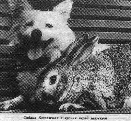
Those to take part in these launches included Otvazhnaya (“Brave One”) who made a flight on July 2nd, 1959, along with a rabbit named Marfusha (“Little Martha”) and another dog named Snezhinka (“Snowflake”). Otvazhnaya would go to make 5 other flights between 1959 and 1960.

Orbital Flights:

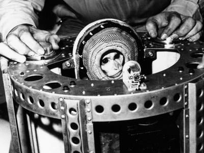
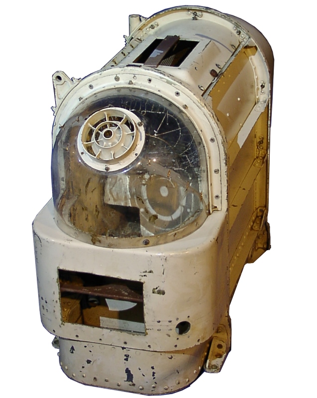
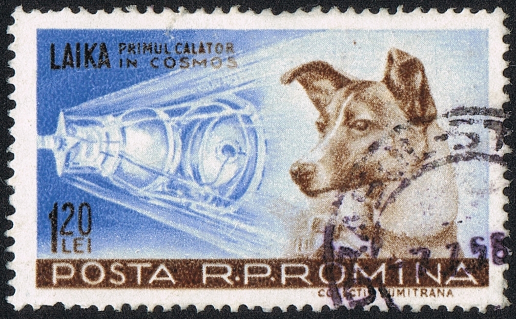
By the late 1950s, and as part of the Sputnik and Vostok programs, Russian dogs began to be sent into orbit around Earth aboard R-7 rockets. On November 3rd, 1957, the famous space dog Laika became the first animal to go into orbit as part of the Sputnik-2 mission. The mission ended tragically, with Laika dying in flight. But unlike other missions where dogs were sent into suborbit, her death was anticipated in advance.

It was believed Laika would survive for a full ten days, when in fact, she died between five and seven hours into the flight. At the time, the Soviet Union claimed she died painlessly while in orbit due to her oxygen supply running out. More recent evidence however, suggests that she died as a result of overheating and panic.

This was due to a series of technical problems which resulted from a botched deployment. The first was the damage that was done to the thermal system during separation, the second was some of the satellite’s thermal insulation being torn loose. As a result of these two mishaps, temperatures in the cabin reached over 40º C.

Animals in Space
The famous space dog Laika, pictured here  before her launch in 1957. Credit: AP Photo/NASA

The mission lasted 162 days before the orbit finally decayed and it fell back to Earth. Her sacrifice has been honored by many countries through a series of commemorative stamps, and she was honored as a “hero of the Soviet Union”. Much was learned from her mission about the behavior of organisms during space flight, though it has been argued that what was learned did not justify the sacrifice.

The next dogs to go into space were Belka (“Squirrel”) and Strelka (“Little Arrow”), which took place on Aug. 19th, 1960, as part of the Sputnik-5 mission. The two dogs were accompanied by a grey rabbit, 42 mice, 2 rats, flies, and several plants and fungi, and all spent a day in orbit before returning safely to Earth.

Strelka went on to have six puppies, one of which was named Pushinka (“Fluffy”). This pup was presented to President John F. Kennedy’s daughter (Caroline) by Nikita Khrushchev in 1961 as a gift. Pushinka went on to have puppies with the Kennedy’s dog (named Charlie), the descendants of which are still alive today.

On Dec. 1st, 1960, space dogs Pchyolka (“Little Bee”) and Mushka (“Little Fly”) went into space as part of Sputnik-6. The dogs, along with another compliment of various test animals, plants and insects, spent a day in orbit. Unfortunately, all died when the craft’s retrorockets experienced an error during reentry, and the craft had to be intentionally destroyed.

The dogs Veterok and Ugoljok who took part in a scientific experiment, 22 day flight in space. Credit: Wikipedia Commons
The dogs Veterok and Ugoljok, who spent 22 days in orbit as part of the Cosmos 110 mission. Credit: Wikipedia Commons/Tekniska museet

Sputnik 9, which launched on March 9th, 1961, was crewed by spacedog Chernenko (“Blackie”) – as well as a cosmonaut dummy, mice and a guinea pig. The capsule made one orbit before returning to Earth and making a soft landing using a parachute. Chernenko was safely recovered from the capsule.

On March 25th, 1961, the dog Zvyozdocha (“Starlet”) who was named by Yuri Gagarin, made one orbit on board the Sputnik-10 mission with a cosmonaut dummy. This practice flight took place a day before Gagarin’s historic flight on April 12th, 1961, in which he became the first man to go into space. After re-entry, Zvezdochka safely landed and was recovered.

Spacedogs Veterok (“Light Breeze”) and Ugolyok (“Coal”) were launched on board a Voskhod space capsule on Feb. 22nd, 1966, as part of Cosmos 110. This mission, which spent 22 days in orbit before safely landing on March 16th, set the record for longest-duration spaceflight by dogs, and would not be broken by humans until 1971.

Legacy:

To this day, the dogs that took part in the Soviet space and cosmonaut training program as seen as heroes in Russia. Many of them, Laika in particular, were put on commemorative stamps that enjoyed circulation in Russia and in many Eastern Bloc countries. There are also monuments to the space dogs in Russia.

Laika, dog launched into space on stamp from Rumania Posta Romania , 1957. Credit: WIkipedia Commons
Romanian commemorate stamp showing Laika, the first dog launched into space, from Rumania Posta, 1957. Credit: Wikipedia Commons

These include the statue that exists outside of Star City, the Cosmonaut training facility in Moscow. Created in 1997, the monument shows Laika positioned behind a statue of a cosmonaut with her ears erect. The Monument to the Conquerors of Space, which was constructed in Moscow in 1964, includes a bas-relief of Laika along with representations of all those who contributed to the Soviet space program.

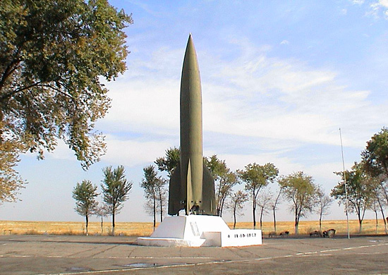
On April 11, 2008, at the military research facility in Moscow where Laika was prepped for her mission to space, officials unveiled a monument of her poised inside the fuselage of a space rocket (shown at top). Because of her sacrifice, all future missions involving dogs and other test animals were designed to be recoverable.

Four other dogs died in Soviet space missions, including Bars and Lisichka (who were killed when their R-7 rocket exploded shortly after launch). On July 28, 1960, Pchyolka and Mushka also died when their space capsule was purposely destroyed after a failed re-entry to prevent foreign powers from inspecting the capsule.

However, their sacrifice helped to advance safety procedures and abort procedures that would be used for many decades to come in human spaceflight.

We have written many interesting articles about animals and space flight here at Universe Today. Here’s Who was the First Dog to go Into Space?, What was the First Animal to go into Space?, What Animals Have been to Space?, Who was “Space Dog” Laika?, and Russian Memorial for Space Dog Laika.

For more information, check out Russian dogs lost in space and NASA’s page about the history of animals in space.

Astronomy Cast has an episode on space capsules.

Sources:

What Does Earth Look like from Mars?

Image taken by the HiRISE camera on NASA's Mars Reconnaissance Orbiter, showing Earth and the Moon. Credit: NASA/JPL

Modern astronomy and space exploration has blessed us with a plethora of wonderful images. Whether they were images of distant planets, stars and galaxies taken by Earth-based telescopes, or close-ups of planets or moons in our own Solar System by spacecraft, there has been no shortage of inspiring pictures. But what would it look like to behold planet Earth from another celestial body?

We all remember the breathtaking photos taken by the Apollo astronauts that showed what Earth looked like from the Moon. But what about our next exploration destination, Mars? With all the robotic missions on or in orbit around the Red Planet, you’d think that there would have been a few occasions where they got a good look back at Earth. Well, as it turn out, they did!

Pictures from Space:

Pictures of Earth have been taken by both orbital missions and surface missions to Mars. The earliest orbiters, which were part of the Soviet Mars and NASA Mariner programs, began arriving in orbit around Mars by 1971. NASA’s Mariner 9 probe was the first to establish orbit around the planet’s (on Nov. 14, 1971), and was also the first spacecraft to orbit another planet.

Image of Earth and Moon, taken by the Mars Orbiter Camera of Mars Global Surveyor on May 8 2003. Credit: NASA/JPL/Malin Space Science Systems

The first orbiter to capture a picture of Earth from Mars, however, was the Mars Global Surveyor, which launched in Nov. 7th, 1996, and arrived in orbit around the planet on Sept. 12th, 1997. In the picture (shown above), which was taken in 2003, we see Earth and the Moon appearing closely together.

At the time the picture was taken, the distance between Mars and Earth was 139.19 million km (86.49 million mi; 0.9304 AU) while the distance between Mars and the Moon was 139.58 million km (86.73 million mi; 0.9330 AU). Interestingly enough, this is what an observer would see from the surface of Mars using a telescope, whereas a naked-eye observer would simply see a single point of light.

Usually, the Earth and Moon are visible as two separate points of light, but at this point in the Moon’s orbit they were too close to resolve with the naked eye from Mars. If you look closely at Earth, you can just make out the shape of South America.

Earth and the Moon, captured by the Mars Express spacecraft on July 3, 2003. Credit: ESA

The picture above was snapped by the Mars Express’s High Resolution Stereo Camera (HRSC) on the ESA’s Mars Express probe. It was also taken in 2003, and is similar in that it shows the Earth and Moon together. However, in this image, we see the two bodies at different points in their orbit – which is why the Moon looks like its farther away. Interestingly enough, this image was actually part of the first data sets to be sent by the spacecraft.

The next orbiter to capture an image of Earth from Mars was the Mars Reconnaissance Orbiter (MRO), which was launched in August of 2005 and attained Martian orbit on March 10th, 2006. When the probe reached Mars, it joined five other active spacecraft that were either in orbit or on the surface, which set a record for the most operational spacecraft in the vicinity of Mars at the same time.

In the course of its mission – which was to study Mars’ surface and weather conditions, as well as scout potential landing sites – the orbiter took many interesting pictures. The one below was taken on Oct. 3rd, 2007, which showed the Earth and the Moon in the same frame.

Mars Reconnaissance Orbiter's High Resolution Imaging Science Experiment (HiRISE) camera can also be used to view other planets. MRO took this image of the Earth and the Moon on 3 October 2007. Credit: NASA/JPL
Image of Earth and the Moon taken by the Mars Reconnaissance Orbiter’s High Resolution Imaging Science Experiment (HiRISE) on Oct. 3rd, 2007. Credit: NASA/JPL

Pictures from the Surface:

As noted already, pictures of Earth have also been taken by robotic missions to the surface of Mars. This has been the case for as long as space agencies have been sending rovers or landers that came equipped with mobile cameras. The earliest rovers to reach the surface – Mars 2 and Mars 3– were both sent by the Soviets.

However, it was not until early March of 2004, while taking photographs of the Martian sky, that the Spirit rover became the first to snap a picture of Earth from the surface of another planet. This image was caught while the rover was attempting to observe Mars’ moon Deimos making a transit of the Sun (i.e. a partial eclipse).

This is something which happens quite often given the moon’s orbital period of about 30 hours. However, on this occasion, the rover managed to also capture a picture of distant Earth, which appeared as little more than a particularly bright star in the night sky.

Earth as seen from Mars, shortly before daybreak. This is the first image of the Earth from the surface of another planet. Credit: NASA/JPL
Earth seen from Mars shortly before daybreak. This is the first image of the Earth from the surface of another planet. Credit: NASA/JPL

The next rover to snap an image of Earth from the Martian surface was Curiosity, which began sending back many breathtaking photos even before it landed on Aug. 6th, 2012. And on Jan. 31st, 2014 – almost a year and a half into its mission – the rover managed to capture an image of both Earth and the Moon in the night sky.

In the image (seen below), Earth and the Moon are just visible as tiny dots to the naked eye – hence the inset that shows them blown up for greater clarity. The distance between Earth and Mars when Curiosity took the photo was about 160 million km (99 million mi).

Earth has been photographed from Mars several times now over the course of the past few decades. Each picture has been a reminder of just how far we’ve come as a species. It also provides us with a preview of what future generations may see when looking out their cabin window, or up at the night sky from other planets.

Image taken by NASA's Curiosity Mars rover, showing Earth and the Moon shining in the night sky. Credit: NASA/JPL
Image taken by NASA’s Curiosity Mars rover, showing Earth and the Moon shining in the night sky. Credit: NASA/JPL

We have written many interesting articles about Earth and Mars here at Universe Today. Here’s Incredible Image of Mars from Earth, Mars Compared to Earth, How Far is Mars from Earth, and How Long Does it Take to get to Mars?

For more information, be sure to check out NASA’s Solar System Exploration page on Mars.

Astronomy Cast also has an interesting episode on the subject – Episode 52: Mars

Sources:

The 2016 Nobel Prize In Physics: It’s Complicated

This year's Nobel Prize in physics highlights the complications of awarding breakthrough achievements. Credit: nobelprize.org

Update: This year’s Nobel Prize in Physics has been awarded to David J. Thouless (University of Washington), F. Duncan M. Haldane (Princeton University), and J. Michael Kosterlitz of Brown University for “theoretical discoveries of topological phase transitions and topological phases of matter”. One half of the prize was awarded to Thouless while the other half was jointly awarded to Haldane and Kosterlitz.

The Nobel Prize in physics is a coveted award. Every year, the prize is bestowed upon the individual who is deemed to have made the greatest contribution to the field of physics during the preceding year. And this year, the groundbreaking discovery of gravitational waves is anticipated to be the main focus.

This discovery, which was announced on February 11th, 2016, was made possible thanks to the development of the Laser Interferometer Gravitational-Wave Observatory (LIGO). As such, it is expected that the three scientists that are most responsible for the invention of the technology will receive the Nobel Prize for their work. However, there are those in the scientific community who feel that another scientist – Barry Barish – should also be recognized.

But first, some background is needed to help put all this into perspective. For starers, gravitational waves are ripples in the curvature of spacetime that are generated by certain gravitational interactions and which propagate at the speed of light. The existence of such waves has been postulated since the late 19th century.

LIGO's two facilities, located in . Credit: ligo.caltech.edu
LIGO’s two observatories, the located in Livingston, Louisiana; and Hanford, Washington. Credit: ligo.caltech.edu

However, it was not until the late 20th century, thanks in large part to Einstein and his theory of General Relativity, that gravitational-wave research began to emerge as a branch of astronomy. Since the 1960s, various gravitational-wave detectors have been built, which includes the LIGO observatory.

Founded as a Caltech/MIT project, LIGO was officially approved by the National Science Board (NSF) in 1984. A decade later, construction began on the facility’s two locations – in Hanford, Washington and Livingston, Louisiana. By 2002, it began to obtain data, and work began on improving its original detectors in 2008 (known as the Advanced LIGO Project).

The credit for the creation of LIGO goes to three scientists, which includes Rainer Weiss, a professor of physics emeritus at the Massachusetts Institute of Technology (MIT); Ronald Drever, an experimental physics who was professor emeritus at the California Institute of Technology and a professor at Glasgow University; and Kip Thorne, the Feynman Professor of Theoretical Physics at Caltech.

In 1967 and 68, Weiss and Thorne initiated efforts to construct prototype detectors, and produced theoretical work to prove that gravitational waves could be successfully analyzed. By the 1970s, using different methods, Weiss and Denver both succeeded in building detectors. In the coming years, all three men remained pivotal and influential, helping to make gravitational astronomy a legitimate field of research.

 A bird's eye view of LIGO Hanford's laser and vacuum equipment area (LVEA). The LVEA houses the pre-stabilized laser, beam splitter, input test masses, and other equipment. Credit: ligo.caltech.edu
LIGO Hanford’s laser and vacuum equipment area (LVEA), which houses the pre-stabilized laser, beam splitter, input test masses, and other equipment. Credit: ligo.caltech.edu

However, it has been argued that without Barish – a particle physicist at Caltech – the discovery would never have been made. Having become the Principal Investigator of LIGO in 1994, he inherited the project at a very crucial time. It had begun funding a decade prior, but coordinating the work of Wiess, Thorne and Drever (from MIT, Caltech and the University of Glasgow, respectively) proved difficult.

As such, it was decided that a single director was needed. Between 1987 and 1994, Rochus Vogt – a professor emeritus of Physics at Caltech – was appointed by the NSF to fill this role. While Vogt brought the initial team together and helped to get the construction of the project approved, he proved difficult when it came to dealing with bureaucracy and documenting his researchers progress.

As such, between 1989 through 1994, LIGO failed to progress technically and organizationally, and had trouble acquiring funding as well. By 1994, Caltech eased Vogt out of his position and appointed Barish to the position of director. Barish got to work quickly, making significant changes to the way LIGO was administered, expanding the research team, and developing a detailed work plan for the NSF.

Barish was also responsible for expanding LIGO beyond its Caltech and MIT constraints. This he did through the creation of the independent LIGO Scientific Collaboration (LSC), which gave access to outside researchers and institutions. This was instrumental in creating crucial partnerships, which included the UK Science and Technology Facilities Council, the Max Planck Society of Germany, and the Australian Research Council.

Artist's impression of how massive bodies (like our Sun) distort space time. Credit: T. Pyle/Caltech/MIT/LIGO Lab
Artist’s impression of how massive bodies (like our Sun) distort space time. Such bodies also create gravity waves when they accelerate through space and time. Credit: T. Pyle/Caltech/MIT/LIGO Lab

By 1999, construction had wrapped up on the LIGO observatories, and by 2002, they began taking their first bits of data. By 2004, the funding and groundwork was laid for the next phase of LIGO development, which involved a multi-year shut-down while the detectors were replaced with improved “Advanced LIGO” versions.

All of this was made possible by Barish, who retired in 2005 to head up other projects. Thanks to his sweeping reforms, LIGO got to work after an abortive start, began to produce data, procured funding, crucial partnerships, and now has more than 1000 collaborators worldwide, thanks to the LSC program he established.

Little wonder then why some scientists think the Nobel Prize should be split four-ways, awarding the three scientists who conceived of LIGO and the one scientist who made it happen. And as Barish himself was quoted as saying by Science:

“I think there’s a bit of truth that LIGO wouldn’t be here if I didn’t do it, so I don’t think I’m undeserving. If they wait a year and give it to these three guys, at least I’ll feel that they thought about it,” he says. “If they decide [to give it to them] this October, I’ll have more bad feelings because they won’t have done their homework.”

The approximate locations of the two gravitational-wave events detected so far by LIGO are shown on this sky map of the southern hemisphere. . Credit: LIGO/Axel Mellinger

However, there is good reason to believe that the award will ultimately be split three ways, leaving Barish out. For instance, Weiss, Drever, and Thorne have been honored three times already this year for their work on LIGO. This has included the Special Breakthrough Prize in Fundamental Physics, the Gruber Cosmology Prize, and Kavli Prize in Astrophysics.

What’s more, in the past, the Nobel Prize in physics has tended to be awarded to those responsible for the intellectual contributions leading to a major breakthrough, rather than to those who did the leg work. Out of the last six Prizes issued (between 2010 and 2015), five have been awarded for the development of experimental methods, observational studies, and theoretical discoveries.

Only one award was given for a technical development. This was the case in 2014 where the award was given jointly to Isamu Akasaki, Hiroshi Amano and Shuji Nakamura for “the invention of efficient blue light-emitting diodes which has enabled bright and energy-saving white light sources”.

Basically, the Nobel Prize is a complicated matter. Every year, it is awarded to those who made a considerable contribution to science, or were responsible for a major breakthrough. But contributions and breakthroughs are perhaps a bit relative. Whom we choose to honor, and for what, can also be seen as an indication of what is valued most in the scientific community.

In the end, this year’s award may serve to highlight how significant contributions do not just entail the development of new ideas and methods, but also in bringing them to fruition.

Further Reading: Science, LIGO, Nobelprize.org

What is Carbon Dating?

Full length negatives of the shroud of Turin. Radiocarbon dating allowed for its true age to be determined. Credit: Wikipedia Commons

Here on Earth, Carbon is found in the atmosphere, the soil, the oceans, and in every living creature. Carbon 12 – aka. C-12, so-named because it has an atomic weight of 12 – is the most common isotope, but it is by no means the only one. Carbon 14 is another, an isotope of carbon that is produced when Nitrogen (N-14) is bombarded by cosmic radiation.

This process causes a proton to be displaced by a neutron, effectively turning atoms of Nitrogen it into an isotope of carbon – known as”radiocarbon”. It is naturally radioactive and unstable, and will therefore spontaneously decay back into N-14 over  a period of time. This property makes it especially useful in a process known as “radiocarbon dating”, or carbon dating for short.

Origin of Radiocarbon:

Radiocarbon enters the biosphere through natural processes like eating and breathing. Plants and animals absorb both C-12 and C-14 in the course of their natural lifetimes simply by carrying out these basic functions. When they die, they cease to consume them, and the isotope of C-14 begins to revert back to its Nitrogen state at an exponential rate due to its radioactive decay.

Comparing the remaining C-14 of a sample to that expected from atmospheric C-14 allows the age of the sample to be estimated. In addition, scientists know that the half-life of radiocarbon is 5,730 years. This means that it takes a sample of radiocarbon 5,730 years for half of it to decay back into nitrogen.

After about 10 half-lives, the amount of radiocarbon left becomes too minuscule to measure and so this technique isn’t particularly reliable for dating specimens which died more than 60,000 years ago – i.e. during the late Middle Paleolithic (aka. Old Stone Age) period.

History of Development:

Experiments that would eventually lead to carbon dating began in the 1939s, thanks to the efforts of the Radiation Laboratory at the University of California, Berkeley. At the time, researchers were attempting to determine if any of the elements common to organic matter had isotopes with half-lives long enough to be of value in biomedical research.

By 1940, the half-life of Carbon 14 was determined, as was the mechanism through which it was created (slow neutrons interacting with Nitrogen in the atmosphere). This contradicted previous work, which held that it was the product of deuterium (H², or heavy hydrogen) and Carbon 13.

A hydrogen atom is made up of one proton and one electron, but its heavy form, called deuterium, also contains a neutron. HDO or heavy water is rare compared to normal drinking water, but being heavier, more likely to stick around when the lighter form vaporizes into space. Credit: NASA/GFSC
A hydrogen atom is made up of one proton and one electron, but its heavy form, called deuterium, also contains a neutron. Credit: NASA/GFSC

During World War II, Willard Libby – a chemist and graduate of Berkeley – read a paper by W. E. Danforth and S. A. Korff (published in 1939) which predicted that C 14 would be created in the atmosphere due to interactions between nitrogen and cosmic rays. From this, Libby came up with the idea of measuring the decay of C 14 as a method of dating organic material.

In 1945, Libby moved to the University of Chicago, where he began the work that would lead to the development of radiocarbon dating. In 1946, he published a paper in which he speculated that C 14 might exist within organic material alongside other carbon isotopes.

After conducting experiments, which measured C-14 in methane derived from sewage samples, Libby and his colleagues were able to demonstrate that organic matter contained radioactive C-14. This was followed by experiments involving wood samples for the tombs of two Egyptian kings, for which the age was known.

Their results proved accurate, with allowances for a small margin of error, and were published in 1949 in the journal Science. In 1960, Libby received the Nobel Prize in Chemistry for this work. Since that time, carbon dating has been used in multiple fields of science, and allowed for key transitions in prehistory to be dated.

Diagram showing how radiocarbon dating works. Credit: howstuffworks.com

Limits of Carbon Dating:

Carbon dating remains limited for a number of reasons. First, there is the assumption that the ratio of C-12 to C-14 in the atmosphere has remained constant, when in fact, the ratio can be affected by a number of factors. For instance, C-14 production rates in the atmosphere, which in turn are affected by the amount of cosmic rays penetrating the Earth’s atmosphere.

This is itself affected by things like the Earth’s magnetic field, which deflects cosmic rays. Furthermore, precise measurements taken over the last 140 years have shown a steady decay in the strength of the Earth’s magnetic field. This means there’s been a steady increase in radiocarbon production (which would increase the ratio).

Another limitation is that this technique can only be applied to organic material such as bone, flesh, or wood, and can’t be used to date rocks directly. On top of that, the addition of Carbon 12 will throw off the ration, thus leading to inaccurate assessments of a sample’s age.

This is where anthropogenic factors come into play. Since fossil fuels have no Carbon 14 content, the burning of gasoline, oil, and other hydrocarbons – and in greater and greater quantity over the course of the past century and a half – has diluted the C-14 content of the atmosphere.

On the other hand, atmospheric testing of nuclear weapons during the 1950s and 1960s is likely to have increased the Carbon 14 content of the atmosphere. In fact, research has been conducted which suggests that nuclear tests may have doubled the concentration of C-14 in this time, compared to natural production by cosmic rays.

Nevertheless, it remains the most accurate means of dating the scientific community has discovered so far. Until such time that another method becomes available – and one that produces smaller margins of error – it will remain the method of choice for archeology, paleontology, and other branches of scientific research.

We have written many articles about Carbon Dating for Universe Today. Here’s How Do We Know How Old Everything Is?, How Old is the Universe?, How Old is the Solar System?, How Long has Humans been on Earth?

If you’d like more info on Carbon Dating, check out NASA’s Virtual Dating: Isochron and Radiocarbon – Geology Labs On-line, and here’s a link to USGS Radiometric Dating Page.

We’ve also recorded an entire episode of Astronomy Cast all about How Carbon Dating Works. Here’s Episode 122: How Old is the Universe? and Episode 164: Inside the Atom.

Sources:

Mercury Is Tectonically Active & Shrinking

New research suggests that Mercury is still contracting and shrinking. Credits: NASA/JHUAPL/Carnegie Institution of Washington/USGS/Arizona State University

Mercury is a fascinating planet. As our Suns’ closest orbiting body, it experiences extremes of heat and cold, has the most eccentric orbit of any Solar planet, and an orbital resonance that makes a single day last as long as two years. But since the arrival of the MESSENGER probe, we have learned some new and interesting things about the planet’s geological history as well.

For example, images that were recently obtained by the NASA spacecraft revealed previously undetected landforms – small fault scarps – that appear to be geologically young. The presence of these features have led scientists to conclude that Mercury is still contracting over time, which means that – like Earth – it is tectonically active.

In geology, fault scarps refer to small step-like formations in the surface of a planet, where one side of a fault has moved vertically relative to the other. Previously, scientists believed that Mercury was tectonically dead, and that all major geological activity had taken place in the planet’s early history.

Small graben, or narrow linear troughs, have been found associated with small fault scarps (lower white arrows) on Mercury, and on Earth’s moon. The small troughs, only tens of meters wide (inset box and upper white arrows), likely resulted from the bending of the crust as it was uplifted, and must be very young to survive continuous meteoroid bombardment. Credits: NASA/JHUAPL/Carnegie Institution of Washington/Smithsonian Institution
Images showing small fault scarps and trough (lower and upper white arrows) found on Mercury;s surface. Credits: NASA/JHUAPL/Carnegie Institution of Washington/Smithsonian Institution

This was evidenced by features spotted by the MESSENGER and Mariner 10 probes, both of which found evidence of large wrinkle ridges and fault scarps on the surface. The features were reasoned to be the result of Mercury contacting as it cooled early in its history (i.e. billion of years ago).

This action caused the planet’s crust to break, forming cliffs up to a kilometer and a half (about 1 mile) in height and hundreds of kilometers long. However, as the MESSENGER team noted, these small scarps were considerably younger, dating to about 50 million years of age.

They concluded that the scarps would have to be this young in order to survive bombardment by comets and meteoroids, a common occurrence on Mercury. They also noted their resemblance to similar features on the Moon, which also has young scarps that are the result of recent contraction.

The team’s findings were reported in a paper titled “Recent Tectonic Activity on Mercury Revealed by Small Thrust Fault Scarps“, which appeared in the October issue of Nature Geoscience.

The MESSENGER spacecraft has been in orbit around Mercury since March 2011. Image Credit: NASA/JHU APL/Carnegie Institution of Washington
The MESSENGER spacecraft has been in orbit around Mercury since March 2011. Credit: NASA/JHU APL/Carnegie Institution of Washington

As Tom Watters, the Smithsonian senior scientist at the National Air and Space Museum and the lead author of the paper, stated in a NASA press release:

“The young age of the small scarps means that Mercury joins Earth as a tectonically active planet, with new faults likely forming today as Mercury’s interior continues to cool and the planet contracts.”

The findings were made during the last 18 months of the MESSENGER mission, during which time the probe lowered its altitude to get higher-resolution images of the planet’s surface. The findings are also consistent with recent findings about Mercury’s global magnetic field, which appears to be powered by the planet’s slowly-cooling outer core.

As Jim Green, NASA’s Planetary Science Director, said of the discovery:

“This is why we explore. For years, scientists believed that Mercury’s tectonic activity was in the distant past. It’s exciting to consider that this small planet – not much larger than Earth’s moon – is active even today.”

All told, these findings have let scientists know that the planet is still alive, in the geological sense. It also means that that there is likely such as thing as Mercury-quakes, something which NASA is sure to follow up on if and when a lander mission (equipped with seismology instruments) is dispatched to the surface of the planet.

Further Reading: NASA, Nature Geoscience

What is a Total Eclipse?

09 March 2016 - Total Solar Eclipse from Palu, Indonesia. Credit and copyright: Justin Ng.

Imagine if you will, that you are a human being living in prehistoric times. You look up at the sky and see the Sun slowly being blocked out,  becoming a ominous black sphere that glows around the edges. Could you really be faulted for thinking that this was some sort of supernatural event, or that the end of the world was nigh?

Of course not. Which is why for thousands of years, human beings believed that solar eclipses were just that – a sign of death or a bad omen. But in fact, an eclipse is merely what happens when one stellar object passes in front of another and obscures it. In astronomy, this happens all the time; and between the Sun, the Moon, and the Earth, total eclipses have been witnessed countless times throughout history.

Definition:

The general term for when one body passes in front of another in a solar system is transit. This term accurately describes how, depending on your vantage point, stellar bodies pass in front of each other on a regular basis, thus causing the reflected light from that body to be temporarily obscured.

However, when we are talking about how the Moon can pass between the Earth and the Sun, and how the Earth can pass between the Sun and the Moon, we use the term eclipse. This is also known as a syzygy, an astronomical term derived from ancient Greek (meaning “yoked together”) that describes a straight-line configuration between three celestial bodies.

Total Solar Eclipse:

When the Moon passes between the Sun and the Earth, and the Moon fully occults (blocks) the Sun, it is known as the solar eclipse. The type of solar eclipse – total or partial – depends on the distance of the Moon from the Earth during the event.

During an eclipse of the Sun, only a thin path on the surface of the Earth is actually able to experience a total eclipse – which is called the path of totality. People on either side of that path see a partial eclipse, where the Sun is only partly obscured by the Moon, relative to those who are standing in the center and witnessing the maximum point of eclipse.

A total solar eclipse occurs when the Earth intersects the Moon’s umbra – i.e. the innermost and darkest part of its shadow. These are relatively brief events, generally lasting only a few minutes, and can only be viewed along a relatively narrow track (up to 250 km wide). The region where a partial eclipse can be observed is much larger.

https://www.flickr.com/photos/auraluu/7085004603/in/photolist-bN5v2M-dufbuU-pzUHQi-nZQkxQ-6KdhJ7-9TLjD4-dtvX13-pidJNx-dtvUxY-dxAA8r-n8uzjn-hx1CzU-du9zKv-c4eHhw-F1szSh-hx2yTc-dv7Y5W-dubgHK-du9zB6-FvPkNQ-drNyGZ-Eg3Msj-F4kfHb-zpuHFU-yUCmvN-yuSXP5-DqsCRp-zfU1bR-zbbFV9-FrtBYE-hdVRQm-rkh8fd-dufbHG-6KGxbK-dufbmf-du9zQe-ryZmAb-FtsHpn-EAUwcK-Ct6Fma-6KLF1b-FiThUB-EEgQjh-E8uHFM-yUC28b-rqtfQ3-yTR8jt-tsa14t-rHcxrz-rXwEhJ
Totality! The view of the last total solar eclipse to cross a U.S. state (Hawaii) back in 1991. Credit and copyright: A. Nartist (shot from Cabo San Lucas, Baja California).

During a solar eclipse, the Moon can sometimes perfectly cover the Sun because its size is nearly the same as the Sun’s when viewed from the Earth. This, of course, is an illusion brought on by the fact that the Moon is much closer to us than the Sun.

And since it is closer, it can block the light from the Sun and cast a shadow on the surface of the Earth. If you’re standing within that shadow, the Sun and the Moon appear to line up perfectly, so that the Moon is completely darkened.

After a solar eclipse reaches totality, the Moon will continue to move past the Sun, obscuring smaller and smaller portions of it and allowing more and more light to pass.

Total Lunar Eclipse:

A total eclipse of the Moon is a different story. In this situation, the entire Moon passes into the Earth’s shadow, darkening it fully. A partial lunar eclipse occurs when the shadow of the Earth doesn’t fully cover the Moon, so only part of the Moon is darkened.

The phases of a total lunar eclipse. Saturday's eclipse will see the briefest totality in a century. Credit: Keith Burns / NASA
The phases of a total lunar eclipse. Saturday’s eclipse will see the briefest totality in a century. Credit: Keith Burns / NASA

Unlike a solar eclipse, a lunar eclipse can be observed from nearly anywhere in an entire hemisphere. In other words, observers all across planet Earth can see this darkening and it appears the same to all. For this reason, total lunar eclipses are much more common and easier to observe from a given location. A lunar eclipse also lasts longer, taking several hours to complete, with totality itself usually averaging anywhere from about 30 minutes to over an hour.

There are three types of lunar eclipses. There’s a penumbral eclipse, when the Moon crosses only the Earth’s penumbra (the region in which only a portion of light is obscured); followed by a partial, when the Moon crosses partially into the Earth’s umbra (where the light is completely blocked).

Last, there is a total eclipse, when the Moon crosses entirely into the Earth’s umbra. A total lunar eclipse involves the Moon passing through all three phases, then gradually passing out of the Earth’s shadow and becoming bright again. Even during a total lunar eclipse, however, the Moon is not completely dark.

Sunlight is still refracted through the Earth’s atmosphere and enters the umbra to provide faint illumination. Similar to what happens during a sunset, the atmosphere scatters shorter wavelength light, causing it to take on a red hue. This is where the phrase ‘Blood Moon‘ comes from.

Since the Moon orbits the Earth, you would expect to see an eclipse of the Sun and the Moon once a lunar month. However, this does not happen simply because the Moon’s orbit isn’t lined up with the Sun. In fact, the Moon’s orbit is tilted by a few degrees – 1.543º between the angle of the ecliptic and the lunar equator, to be exact.

This means that three objects only have the opportunity to line up and cause an eclipse a few times a year. It’s possible for a total of 7 solar and lunar eclipses every year, but that only happens a few times every century.

Other Types of Eclipses:

The term eclipse is most often used to describe a conjunction between the Earth, Sun and Moon. However, it can also refer to such events beyond the Earth–Moon system. For example, a planet moving into the shadow of one of its moons, a moon passing into the shadow of its host planet, or a moon passing into the shadow of another moon.

Mosaic of Saturn seen in eclipse in September 2006. Earth is the bright dot just inside the F ring at upper left. (CICLOPS/NASA/JPL-Caltech/SSI)

For instance, during the Apollo 12 mission in 1969, the crew was able to observe the Sun being eclipsed by the Earth. In 2006, during its mission to study Saturn, the Cassini spacecraft was able to capture the image above, which shows the gas giant transiting between the probe and the Sun.

In July of 2015, when the New Horizons mission passed through the shadow of Pluto, it was able to capture a stunning image of the dwarf planet eclipsing the Sun. The image was taken at a distance of about 2 million km (1.25 million miles), which provided the necessary vantage point to see the disc of the Sun become fully obscured.

On top of that, many other bodies in the Solar System can experience eclipses as well. These include the four gas giants, all of which have major moons that periodically transit between the planet and either Earth-based or space-based observatories.

The most impressive and common of these involve Jupiter and its four largest moons (Io, Europa, Ganymede and Callisto). Given the size and low axial tilt of these moons, they often experience eclipses with Jupiter as a result of transits, relative to our instruments.

An enviable view, of the most distant eclipse seen yet, as New Horizons flies through the shadow of Pluto. Image credit: NASA/JPL.
An enviable view, of the most distant eclipse seen yet, as New Horizons flies through the shadow of Pluto. Credit: NASA/JPL.

A well-known example occurred in April of 2014, when the Hubble Space Telescope caught an image of Ganymede passing in front at of Jupiter. At the time the image was taken, Ganymede was casting its shadow within Jupiter’s Great Red Spot, which lent the planet a cyclops-like appearance (see below).

The other three gas giants are known to experiences eclipses as well. However, these only occur at certain periods the planet’s orbit of the Sun, due to their higher inclination between the orbits of their moons and the orbital plane of the planets. For instance, Saturn’s largest moon Titan has been known to only occult the ringed gas giant once about every 15 years.

Pluto has also been known to experience eclipses with is largest moon (and co-orbiting body) Charon. However, in all of these cases, the eclipses are never total, as they do not have the size to obscure the much larger gas giant. Instead, the passage of the moons in front of the larger celestial bodies either cast small shadows on the cloud tops of the gas giants, or lead to an annular eclipse at most.

Similarly, on Mars, only partial solar eclipses are ever possible. This is because Phobos or Deimos are not large enough (or distant enough in their orbits) to cover the Sun’s disc, as seen from the surface of the planet. Phobos and Deimos have also been known to experience lunar eclipses as they slip into the shadow of Mars.

Jupiter's Great Red Spot and Ganymede's Shadow. Image Credit: NASA/ESA/A. Simon (Goddard Space Flight Center)
Jupiter’s Great Red Spot and Ganymede’s Shadow. Image Credit: NASA/ESA/A. Simon (Goddard Space Flight Center)

Martian eclipses have been photographed numerous times from both the surface and from orbit. For example, in 2010, the Spirit rover captured images of a Martian lunar eclipse as Phobos, the larger of the two martian moons, was photographed while slipping into the shadow of Mars.

Also, between Nov. 4 and Nov. 5, 2010, the Opportunity rover captured several images (later turned into movies) of a Martian sunset. In the course of imaging the Sun for a total of 17 minutes, Opportunity captured stills of the Sun experiencing a solar eclipse. And on September 13th, 2012 – during the 37th day of its mission (Sol 27) – the Curiosity rover captured an image of Phobos transiting the Sun.

As far as astronomical events go, total eclipses (Lunar and Solar) are not uncommon occurrences. If you ever want to witness a one, all you need to do is keep track of when one will be visible from your part of the world. Some good resources for this are NASA’s Eclipse Website and timeanddate.com.

Or, if you’re the really adventurous type, you can find out where on Earth the next path of totality is going to be, and then book a vacation to go there. Get to the right spot at the right time, and you should be getting the view of a lifetime!

We have written many articles about the eclipse for Universe Today. Here’s a list of articles about specific times when a total Lunar Eclipse took place, and here’s a list of Solar Eclipse articles. And be sure to check out this article and video of an Annular Eclipse.

If you’d like more info about the Eclipse, check out NASA Homepage, and here’s a link to NASA’s Solar System Simulator.

We’ve also recorded related episodes of Astronomy Cast about Eclipses. Listen here, Episode 160: Eclipses.

Sources:

Europa’s Venting Global Ocean May Be Easier To Reach Than We Thought

Artist's impression of a water vapor plume on Europa. Credit: NASA/ESA/K. Retherford/SWRI

Last week, on Tuesday, September 20th, NASA announced that they had made some interesting findings about Jupiter’s icy moon Europa. These were based on images taken by the Hubble Space Telescope, the details of which would be released on the following week. Needless to say, since then, the scientific community and general public have been waiting with baited breath.

Earlier today (September 26th) NASA put an end to the waiting and announced the Hubble findings during a NASA Live conference. According to the NASA panel, which was made up of members of the research team, this latest Europa-observing mission revealed evidence of plumes of saline water emanating from Europa’s surface. If true, this would mean that the moon’s subsurface ocean would be more accessible than previously thought.

Using Hubble’s Space Telescope Imaging Spectrograph (STIS) instrument, the team conducted observations of Jupiter and Europa in the ultra-violet spectrum over the course of 15 months. During that time, Europa passed in front of Jupiter (occulted the gas giant) on 10 separate occasions.

And on three of these occasions, the team saw what appeared to be plumes of water erupting from the surface. These plumes were estimated to be reaching up to 200 km (125 miles) from the southern region of Europa before (presumably) raining back onto the surface, depositing water ice and material from the interior.

The purpose of the observation was to examine Europa’s possible extended atmosphere (aka. exosphere). The method the team employed was similar to the one used to detect atmospheres around extra-solar planets. As William Sparks of the Space Telescope Science Institute (STScI) in Baltimore (and the team leader), explained in a NASA press release:

“The atmosphere of an extrasolar planet blocks some of the starlight that is behind it. If there is a thin atmosphere around Europa, it has the potential to block some of the light of Jupiter, and we could see it as a silhouette. And so we were looking for absorption features around the limb of Europa as it transited the smooth face of Jupiter.”

When they looked at Europa using this same technique, they noted that small patches on the surface were dark, indicating the absorption of UV light. This corresponded to previous work done by Lorenz Roth (of the Southwest Research Institute) and his team of researchers in 2012. At this time, they detected evidence of water vapor coming from Europa’s southern polar region.

Europa transit illustration. Europa orbits Jupiter every 3 and a half days, and on every orbit it passes in front of Jupiter, raising the possibility of plumes being seen as silhouettes absorbing the background light of Jupiter. Credits: A. Field (STScI)

As they indicated in a paper detailing their results – titled “Transient Water Vapor at Europa’s South Pole” – Roth’s team also relied on UV observations made using the Hubble telescope. Noting a statistically coincident amount of hydrogen and oxygen emissions, they concluded that this was the result of ejected water vapor being broken apart by Jupiter’s radiation (a process known as radiolysis).

Though their methods differed, Sparks and his research team also found evidence of these apparent water plumes, and in the same place no less. Based on the latest information from STIS, most of the apparent plumes are located in the moon’s southern polar region while another appears to be located in the equatorial region.

“When we calculate in a completely different way the amount of material that would be needed to create these absorption features, it’s pretty similar to what Roth and his team found,” Sparks said. “The estimates for the mass are similar, the estimates for the height of the plumes are similar. The latitude of two of the plume candidates we see corresponds to their earlier work.”

Another interesting conclusion to come from this and the 2012 study is the likelihood that these water plumes are intermittent. Basically, Europa is tidally-locked world, which means the same side is always being presented to us when it transits Jupiter. This occus once every 3.5 days, thus giving astronomers and planetary scientists plenty of viewing opportunities.

 This composite image shows suspected plumes of water vapor erupting at the 7 o’clock position off the limb of Jupiter’s moon Europa. The Hubble data were taken on January 26, 2014. Credit: Credits: NASA/ESA/W. Sparks (STScI)/USGS Astrogeology Science Center
This composite image shows suspected plumes of water vapor erupting at the 7 o’clock position off the limb of Jupiter’s moon Europa. The Hubble data were taken on January 26, 2014. Credit: Credits: NASA/ESA/W. Sparks (STScI)/USGS Astrogeology Science Center

But the fact that plumes have been observed at some points and not others would seem to indicate that they are periodic. In addition, Roth’s team attempted to spot one of the plume’s observed by Sparks and his colleagues a week after they reported it. However, they were unable to locate this supposed water source. As such, it would appear that the plumes, if they do exist, are short-lived.

These findings are immensely significant for two reasons. On the one hand, they are further evidence that a warm-water, saline ocean exists beneath Europa’s icy surface. On the other, they indicate that any future mission to Europa would be able to access this salt-water ocean with greater ease.

Ever since the Galileo spacecraft conducted a flyby of the Jovian moon, scientists have believed that an interior ocean is lying beneath Europa’s icy surface – one that has between two and three times as much water as all of Earth’s oceans combined. However, estimates of the ice’s thickness range from it being between 10 to 30 km (6–19 mi) thick – with a ductile “warm ice” layer that increases its total thickness to as much as 100 km (60 mi).

Knowing the water periodically reaches the surface through fissures in the ice would mean that any future mission (which would likely include a submarine) would not have to drill so deep. And considering that Europa’s interior ocean is considered to be one of our best bets for finding extra-terrestrial life, knowing that the ocean is accessible is certainly exciting news.

A comparison of 2014 transit and 2012 Europa aurora observations. The raw transit image, left, has dark fingers or patches of possible absorption in the same place that a different team (led by Lorenz Roth) found auroral emission from hydrogen and oxygen, the dissociation products of water. Credits: NASA, ESA, W. Sparks (left image) L. Roth (right image)
A comparison of 2014 transit and 2012 Europa aurora observations. Credits: NASA, ESA, W. Sparks (left image) L. Roth (right image)

And the news is certainly causing its fair share of excitement for the people who are currently developing NASA’s proposed Mission to Europa, which is scheduled to launch sometime in the 2020s. As Dr. Cynthia B. Phillips, a Staff Scientist and the Science Communications Lead for the Europa Project, told Universe Today via email:

“This new discovery, using Hubble Space Telescope data, is an intriguing data point that helps lend support to the idea that there are active plumes on Europa today. While not an absolute confirmation, the new Sparks et al. result, in combination with previous observations by Roth et al. (also using HST but with a different technique), is consistent with the presence of intermittent plumes ejecting water vapor from the Southern Hemisphere of Europa. Such observations are difficult to perform from Earth, however, even with Hubble, and thus these results remain inconclusive.

“Confirming the presence or absence of plumes on Europa, as well as investigating many other mysteries of this icy ocean world, will require a dedicated spacecraft in the Jupiter system.   NASA currently plans to send a multiple-flyby spacecraft to Europa, which would make many close passes by Europa in the next decade. The spacecraft’s powerful suite of scientific instruments will be able to study Europa’s surface and subsurface in unprecedented detail, and if plumes do exist, it will be able to observe them directly and even potentially measure their composition.  Until the Europa spacecraft is in place, however, Earth-based observations such as the new Hubble Space Telescope results will remain our best technique to observe Jupiter’s mysterious moon.”

Naturally, Sparks was clear that this latest information was not entirely conclusive. While he believes that the results were statistically significant, and that there were no indications of artifacts in the data, he also emphasized that observations conducted in the UV wavelength are tricky. Therefore, more evidence is needed before anything can be said definitively.

In the future, it is hoped that future observation will help to confirm the existence of water plumes, and how these could have helped create Europa’s “chaos terrain”. Future missions, like NASA’s James Webb Space Telescope (scheduled to launch in 2018) could help confirm plume activity by observing the moon in infrared wavelengths.

As Paul Hertz, the director of the Astrophysics Division at NASA Headquarters in Washington, said:

“Hubble’s unique capabilities enabled it to capture these plumes, once again demonstrating Hubble’s ability to make observations it was never designed to make. This observation opens up a world of possibilities, and we look forward to future missions — such as the James Webb Space Telescope — to follow up on this exciting discovery.”

Other team members include Britney Schmidt, an assistant professor at the School of Earth and Atmospheric Sciences at Georgia Institute of Technology in Atlanta; and Jennifer Wiseman, senior Hubble project scientist at NASA’s Goddard Space Flight Center in Greenbelt, Maryland. Their work will be published in the Sept. 29 issue of the Astrophysical Journal.

And be sure to enjoy this video by NASA about this exciting find:

Further Reading: NASA Live

How Can You see the Northern Lights?

Aurora borealis in Fairbanks, AK. on Monday night March 16. Credit: John Chumack

The Northern Lights have fascinated human beings for millennia. In fact, their existence has informed the mythology of many cultures, including the Inuit, Northern Cree, and ancient Norse. They were also a source of intense fascination for the ancient Greeks and Romans, and were seen as a sign from God by medieval Europeans.

Thanks to the birth of modern astronomy, we now know what causes both the Aurora Borealis and its southern sibling – Aurora Australis. Nevertheless, they remain the subject of intense fascination, scientific research, and are a major tourist draw. For those who live north of 60° latitude, this fantastic light show is also a regular occurrence.

Causes:

Aurora Borealis (and Australis) is caused by interactions between energetic particles from the Sun and the Earth’s magnetic field. The invisible field lines of Earth’s magnetoshere travel from the Earth’s northern magnetic pole to its southern magnetic pole. When charged particles reach the magnetic field, they are deflected, creating a “bow shock” (so-named because of its apparent shape) around Earth.

However, Earth’s magnetic field is weaker at the poles, and some particles are therefore able to enter the Earth’s atmosphere and collide with gas particles in these regions. These collisions emit light that we perceive as wavy and dancing, and are generally a pale, yellowish-green in color.

The variations in color are due to the type of gas particles that are colliding. The common yellowish-green is produced by oxygen molecules located about 100 km (60 miles) above the Earth, whereas high-altitude oxygen – at heights of up to 320 km (200 miles) – produce all-red auroras. Meanwhile, interactions between charged particles and nitrogen will produces blue or purplish-red auroras.

Variability:

The visibility of the northern (and southern) lights depends on a lot of factors, much like any other type of meteorological activity. Though they are generally visible in the far northern and southern regions of the globe, there have been instances in the past where the lights were visible as close to the equator as Mexico.

In places like Alaska, Norther Canada, Norway and Siberia, the northern lights are often seen every night of the week in the winter. Though they occur year-round, they are only visible when it is rather dark out. Hence why they are more discernible during the months where the nights are longer.

The magnetic field and electric currents in and around Earth generate complex forces that have immeasurable impact on every day life. The field can be thought of as a huge bubble, protecting us from cosmic radiation and charged particles that bombard Earth in solar winds. It’s shaped by winds of particles blowing from the sun called the solar wind, the reason it’s flattened on the “sun-side” and swept out into a long tail on the opposite side of the Earth. Credit: ESA/ATG medialab
The magnetic field and electric currents in and around Earth generate complex forces, and also lead to the phenomena known as aurorae. Credit: ESA/ATG medialab

Because they depend on the solar wind, auroras are more plentiful during peak periods of activity in the Solar Cycle. This cycle takes places every 11 years, and is marked by the increase and decrease of sunspots on the sun’s surface. The greatest number of sunspots in any given solar cycle is designated as a “Solar Maximum“, whereas the lowest number is a “Solar Minimum.”

A Solar Maximum also accords with bright regions appearing in the Sun’s corona, which are rooted in the lower sunspots. Scientists track these active regions since they are often the origin of eruptions on the Sun, such as solar flares or coronal mass ejections.

The most recent solar minimum occurred in 2008. As of January 2010, the Sun’s surface began to increase in activity, which began with the release of a lower-intensity M-class flare. The Sun continued to get more active, culminating in a Solar Maximum by the summer of 2013.

Locations for Viewing:

The ideal places to view the Northern Lights are naturally located in geographical regions north of 60° latitude.  These include northern Canada, Greenland, Iceland, Scandinavia, Alaska, and Northern Russia. Many organizations maintain websites dedicated to tracking optimal viewing conditions.

The camera recorded pale purple and red but the primary color visible to the eye was green. Credit: Bob Kin
An image captured of the northern lights, which appear pale purple and red, though the primary color visible to the eye was green. Credit: Bob Kin

For instance, the Geophysical Institute of the University of Alaska Fairbanks maintains the Aurora Forecast. This site is regularly updated to let residents know when auroral activity is high, and how far south it will extend. Typically, residents who live in central or northern Alaska (from Fairbanks to Barrow) have a better chance than those living in the south (Anchorage to Juneau).

In Northern Canada, auroras are often spotted from the Yukon, the Northwest Territories, Nunavut, and Northern Quebec. However, they are sometimes seen from locations like Dawson Creek, BC; Fort McMurry, Alberta; northern Saskatchewan and the town of Moose Factory by James Bay, Ontario. For information, check out Canadian Geographic Magazine’s “Northern Lights Across Canada“.

The National Oceanic and Atmospheric Agency also provides 30 minute forecasts on auroras through their Space Weather Prediction Center. And then there’s Aurora Alert, an Android App that allows you to get regular updates on when and where an aurora will be visible in your region.

Understanding the scientific cause of auroras has not made them any less awe-inspiring or wondrous. Every year, countless people venture to locations where they can be seen. And for those serving aboard the ISS, they got the best seat in the house!

Speaking of which, be sure to check out this stunning NASA video which shows the Northern Lights being viewed from the ISS:

We have written many interesting articles about Auroras here at Universe Today. Here’s The Northern and Southern Lights – What is an Aurora?, What is the Aurora Borealis?, What is the Aurora Australis?, What Causes the Northern Lights?, How Does the Aurora Borealis Form?, and Watch Fast and Furious All-sky Aurora Filmed in Real Time.

For more information, visit the THEMIS website – a NASA mission that is currently studying space weather in great detail. The Space Weather Center has information on the solar wind and how it causes aurorae.

Astronomy Cast also has episodes on the subject, like Episode 42: Magnetism Everywhere.

Sources:

Why Are Stars Different Colors?

Artist's impression of a white dwarf star in orbit around Sirius (a white supergiant). Credit: NASA, ESA and G. Bacon (STScI)

Stars are beautiful, wondrous things. Much like planets, planetoids and other stellar bodies, they come in many sizes, shapes, and even colors. And over the course of many centuries, astronomers have come to discern several different types of stars based on these fundamental characteristics.

For instance, the color of a star – which varies from bluish-white and yellow to orange and red – is primarily due to its composition and effective temperature. And at all times, stars emit light which is a combination of several different wavelengths. On top of that, the color of a star can change over time.

Composition:

Different elements emit different wavelengths of electromagnetic radiation when heated. In the case of stars, his includes its main constituents (hydrogen and helium), but also the various trace elements that make it up. The color that we see is the combination of these different electromagnetic wavelengths, which are referred to as as a Planck’s curve.

Diagram illustrating Wein's Law (colored curves), which describes the emission of radiation from a black body. Credit: Wikipedia Commons/Darth Kule
Diagram illustrating Wein’s Law, which describes the emission of radiation from a black body based on its peak wavelength. Credit: Wikipedia Commons/Darth

The wavelength at which a star emits the most light is called the star’s “peak wavelength” (which known as Wien’s Law), which is the peak of its Planck curve. However, how that light appears to the human eye is also mitigated by the contributions of the other parts of its Planck curve.

In short, when the various colors of the spectrum are combined, they appear white to the naked eye. This will make the apparent color of the star appear lighter than where star’s peak wavelength falls on the color spectrum. Consider our Sun. Despite the fact that its peak emission wavelength corresponds to the green part of the spectrum, its color appears pale yellow.

A star’s composition is the result of its formation history. Ever star is born of a nebula made up of gas and dust, and each one is different. While nebulas in the interstellar medium are largely composed of hydrogen, which is the main fuel for star creation, they also carry other elements. The overall mass of the nebula, as well as the various elements that make it up, determine what kind of star will result.

The change in color these elements add to stars is not very obvious, but can be studied thanks to the method known as spectroanalysis. By examining the various wavelengths a star produces using a spectrometer, scientists are able to determine what elements are being burned inside.

Temperature and Distance:

The other major factor effecting a star’s color is its temperature. As stars increase in heat, the overall radiated energy increases, and the peak of the curve moves to shorter wavelengths. In other words, as a star becomes hotter, the light it emits is pushed further and further towards the blue end of the spectrum. As stars grow colder, the situation is reversed (see below).

A third and final factor that will effect what light a star appears to be emitting is known as the Doppler Effect. When it comes to sound, light, and other waves, the frequency can increase or decrease based on the distance between the source and the observer.

When it comes to astronomy, this effect causes the what is known as “redshift” and “blueshift” – where the visible light coming from a distant star is shifted towards the red end of the spectrum if it is moving away, and the blue end if it is moving closer.

Modern Classification:

Modern astronomy classifies stars based on their essential characteristics, which includes their spectral class (i.e. color), temperature, size, and brightness. Most stars are currently classified under the Morgan–Keenan (MK) system, which classifies stars based on temperature using the letters O, B, A, F, G, K, and M, – O being the hottest and M the coolest.

Each letter class is then subdivided using a numeric digit with 0 being hottest and 9 being coolest (e.g. O1 to M9 are the hottest to coldest stars). In the MK system, a luminosity class is added using Roman numerals. These are based on the width of certain absorption lines in the star’s spectrum (which vary with the density of the atmosphere), thus distinguishing giant stars from dwarfs.

Luminosity classes 0 and I apply to hyper- or supergiants; classes II, III and IV apply to bright, regular giants, and subgiants, respectively; class V is for main-sequence stars; and class VI and VII apply to subdwarfs and dwarf stars. There is also the Hertzsprung-Russell diagram, which relates stellar classification to absolute magnitude (i.e. intrinsic brightness), luminosity, and surface temperature.

The same classification for spectral types are used, ranging from blue and white at one end to red at the other, which is then combined with the stars Absolute Visual Magnitude (expressed as Mv) to place them on a 2-dimensional chart (see below).

The Hertzspirg-Russel diagram, showing the relation between star's color, AM. luminosity, and temperature. Credit: astronomy.starrynight.com
The Hertzspirg-Russel diagram, showing the relation between star’s color, AM. luminosity, and temperature. Credit: astronomy.starrynight.com

On average, stars in the O-range are hotter than other classes, reaching effective temperatures of up to 30,000 K. At the same time, they are also larger and more massive, reaching sizes of over 6 and a half solar radii and up to 16 solar masses. At the lower end, K and M type stars (orange and red dwarfs) tend to be cooler (ranging from 2400 to 5700 K), measuring 0.7 to 0.96 times that of our Sun, and being anywhere from 0.08 to 0.8 as massive.

Stellar Evolution:

Stars also go through an evolutionary life cycle, during which time their sizes, temperatures and colors change. For example, when our Sun exhausts all the hydrogen in its the core, it will become unstable and collapse under its own weight. This will cause the core to heat up and get denser, causing the Sun to grow in size.

At this point, it will have left its Main Sequence phase and entered into the Red Giant Phase of its life, which (as the name would suggest) will be characterized by expansion and it becoming a deep red. When this happens, it is theorized that our Sun will expand to encompass the orbits of Mercury and even Venus.

Earth, if it survives this expansion, will be so close that it will be rendered uninhabitable. When our Sun then reaches its post-Red Giant Phase, the Sun will begin to eject mass, leaving an exposed core known as a white dwarf. This remnant will survive for trillions of years before fading to black.

This is believed to be the case with all stars that have between 0.5 to 1 Solar Mass (half, or as much mass of our Sun). The situation is slightly different when it comes to low mass stars (i.e. red dwarfs), which typically have around 0.1 Solar Masses.

It is believed that these stars can remain in their Main Sequence for some six to twelve trillion years and will not experience a Red Giant Phase. However, they will gradually increase in both temperature and luminosity, and will exist for several hundred billion more years before they eventually collapse into a white dwarf.

On the other hand, supergiant stars (up to 100 Solar Masses or more) have so much mass in their cores that they will likely experience helium ignition as soon as they exhaust their supplies of hydrogen. As such, they will likely not survive to become Red Supergiants, and will instead end their lives in a massive supernova.

To break it all down, stars vary in color depending on their chemical compositions, their respective sizes and their temperatures. Over time, as these characteristics change (as a result of them spending their fuel) many will darken and become redder, while others will explode magnificently. The more stars observe, the more we come to know about our Universe and its long, long history!

We have written many articles about stars on Universe Today. Here’s What is the Biggest Star in the Universe?, What is a Binary Star?, Do Stars Move?, What are the Most Famous Stars?, What is the Brightest Star in the Sky, Past and Future?

Want more information on stars? Here’s Hubblesite’s News Releases about Stars, and more information from NASA’s imagine the Universe.

We have recorded several episodes of Astronomy Cast about stars. Here are two that you might find helpful: Episode 12: Where Do Baby Stars Come From, and Episode 13: Where Do Stars Go When they Die?

Sources:

What is a Debris Flow?

Landslide in Guatemala

Landslides constitute one of the most destructive geological hazards in the world today. One of the main reasons for this is because of the high speeds that slides can reach, up to 160 km/hour (100 mph). Another is the fact that these slides can carry quite a bit of debris with them that serve to amplify their destructive force.

Taken together, this is what is known as a Debris Flow, a natural hazard that can take place in many parts of the world. A single flow is capable of burying entire towns and communities, covering roads, causing death and injury, destroying property and bringing all transportation to a halt. So how do we deal with them?

Definition:

A Debris Flow is basically a fast-moving landslide made up of liquefied, unconsolidated, and saturated mass that resembles flowing concrete. In this respect, they are not dissimilar from avalanches, where unconsolidated ice and snow cascades down the surface of a mountain, carrying trees and rocks with it.

Images of a Debris Flow Chute and Deposit, taken by the Arizona Geological Survey (AZGS). Credit: azgs.com
Images of a Debris Flow Chute
and Deposit, taken by the Arizona Geological Survey (AZGS). Credit: azgs.com

A common misconception is to confuse debris flows with landslides or mudflows. In truth, they differ in that landslides are made up of a coherent block of material that slides over surfaces. Debris flows, by contrast, are made up of “loose” particles that move independently within the flow.

Similarly, mud flows are composed of mud and water, whereas debris flows are made up larger particles. All told, it has been estimated that at least 50% of the particles contained within a debris flow are made-up of sand-sized or larger particles (i.e. rocks, trees, etc).

Types of Flows:

There are two types of debris flows, known as Lahar and Jökulhlaup. The word Lahar is Indonesian in origin and has to do with flows that are related to volcanic activity. A variety of factors may trigger a lahar, including melting of glacial ice due to volcanic activity, intense rainfall on loose pyroclastic material, or the outbursting of a lake that was previously dammed by pyroclastic or glacial material.

Jökulhlaup is an Icelandic word which describes flows that originated from a glacial outburst flood. In Iceland, many such floods are triggered by sub-glacial volcanic eruptions, since Iceland sits atop the Mid-Atlantic Ridge. Elsewhere, a more common cause of jökulhlaups is the breaching of ice-dammed or moraine-dammed lakes.

Debris flow channel in Ladakh, NW Indian Himalaya, produced in the storms of August 2010. Credit: Wikipedia Commons/DanHobley
Debris flow channel in Ladakh, near the northwestern Indian Himalaya, produced in the storms of August 2010. Credit: Wikipedia Commons/DanHobley

Such breaching events are often caused by the sudden calving of glacier ice into a lake, which then causes a displacement wave to breach a moraine or ice dam. Downvalley of the breach point, a jökulhlaup may increase greatly in size by picking up sediment and water from the valley through which it travels.

Causes of Flows:

Debris flows can be triggered in a number of ways. Typically, they result from sudden rainfall, where water begins to wash material from a slope, or when water removed material from a freshly burned stretch of land. A rapid snowmelt can also be a cause, where newly-melted snow water is channeled over a steep valley filled with debris that is loose enough to be mobilized.

In either case, the rapidly moving water cascades down the slopes and into the canyons and valleys below, picking up speed and debris as it descends the valley walls. In the valley itself, months’ worth of built-up soil and rocks can be picked up and then begin to move with the water.

As the system gradually picks up speed, a feedback loop ensues, where the faster the water flows, the more it can pick up. In time, this wall begins to resemble concrete in appearance but can move so rapidly that it can pluck boulders from the floors of the canyons and hurl them along the path of the flow. It’s the speed and enormity of these carried particulates that makes a debris flow so dangerous.

Deforestation (like this clearcut in Sumatra, Indonesia) can result in debris flows. Credit: worldwildlife.org

Another major cause of debris flows is the erosion of steams and riverbanks. As flowing water gradually causes the banks to collapse, the erosion can cut into thick deposits of saturated materials stacked up against the valley walls. This erosion removes support from the base of the slope and can trigger a sudden flow of debris.

In some cases, debris flows originate from older landslides. These can take the form of unstable masses perched atop a steep slope. After being lubricated by a flow of water over the top of the old landslide, the slide material or erosion at the base can remove support and trigger a flow.

Some debris flows occur as a result of wildfires or deforestation, where vegetation is burned or stripped from a steep slope. Prior to this, the vegetation’s roots anchored the soil and removed absorbed water. The loss of this support leads to the accumulation of moisture which can result in structural failure, followed by a flow.

Sarychev volcano, (located in Russia's Kuril Islands, northeast of Japan) in an early stage of eruption on June 12, 2009. Credit: NASA
Sarychev volcano, (located in Russia’s Kuril Islands, northeast of Japan) in an early stage of eruption on June 12, 2009. Credit: NASA

A volcanic eruption can flash melt large amounts of snow and ice on the flanks of a volcano. This sudden rush of water can pick up ash and pyroclastic debris as it flows down the steep volcano and carry them rapidly downstream for great distances.

In the 1877 eruption of Cotopaxi Volcano in Ecuador, debris flows traveled over 300 kilometers down a valley at an average speed of about 27 kilometers per hour. Debris flows are one of the deadly “surprise attacks” of volcanoes.

Prevention Methods:

Many methods have been employed for stopping or diverting debris flows in the past. A popular method is to construct debris basins, which are designed to “catch” a flow in a depressed and walled area. These are specifically intended to protect soil and water sources from contamination and prevent downstream damage.

Some basins are constructed with special overflow ducts and screens, which allow the water to trickle out from the flow while keeping the debris in place, while also allowing for more room for larger objects. However, such basins are expensive, and require considerable labor to build and maintain; hence why they are considered an option of last resort.

Aerial view of debris-flow deposition resulting in widespread destruction on the Caraballeda fan of the Quebrada San Julián. Credit: US Geological Survey
Aerial view of the destruction caused by a debris-flow in the Venezuelan town of Caraballeda. Credit: US Geological Survey

Currently, there is no way to monitor for the possibility of debris flow, since they can occur very rapidly and are often dependent on cycles in the weather that can be unpredictable. However, early warning systems are being developed for use in areas where debris flow risk is especially high.

One method involves early detection, where sensitive seismographs detect debris flows that have already started moving and alert local communities. Another way is to study weather patterns using radar imaging to make precipitation estimates – using rainfall intensity and duration values to establish a threshold of when and where a flows might occur.

In addition, replanting forests on hillsides to anchor the soil, as well as monitoring hilly areas that have recently suffered from wildfires is a good preventative measure. Identifying areas where debris flows have happened in the past, or where the proper conditions are present, is also a viable means of developing a debris flow mitigation plan.

We have written many articles about landslides for Universe Today. Here’s Satellites Could Predict Landslides, Recent Landslide on Mars, More Recent Landslides on Mars, Landslides and Bright Craters on Ceres Revealed in Marvelous New Images from Dawn.

If you’d like more info on debris flow, check out Visible Earth Homepage. And here’s a link to NASA’s Earth Observatory.

We’ve also recorded an episode of Astronomy Cast all about planet Earth. Listen here, Episode 51: Earth.

Sources: