David Dickinson, Author at Universe Today

May 13, 2014December 23, 2015 by David Dickinson

14 Red Dwarf Stars to View with Backyard Telescopes

An artist's conception of a red dwarf solar system. Credit: NASA/JPL-Caltech.

They’re nearby, they’re common and — at least in the latest exoplanet newsflashes hot off the cyber-press — they’re hot. We’re talking about red dwarf stars, those “salt of the galaxy” stars that litter the Milky Way. And while it’s true that there are more of “them” than there are of “us,” not a single one is bright enough to be seen with the naked eye from the skies of Earth.

A reader recently brought up an engaging discussion of what red dwarfs might be within reach of a backyard telescope, and thus this handy compilation was born.

Of course, red dwarfs are big news as possible hosts for life-bearing planets. Though the habitable zones around these stars would be very close in, these miserly stars will shine for trillions of years, giving evolution plenty of opportunity to do its thing. These stars are, however, tempestuous in nature, throwing out potentially planet sterilizing flares.

Red dwarf stars range from about 7.5% the mass of our Sun up to 50%. Our Sun is very nearly equivalent 1000 Jupiters in mass, thus the range of red dwarf stars runs right about from 75 to 500 Jupiter masses.

For this list, we considered red dwarf stars brighter than +10^th magnitude, with the single exception of 40 Eridani C as noted.

The closest stars within 14 light years of our solar system. Credit: Wikimedia Commons, Public Domain graphic.

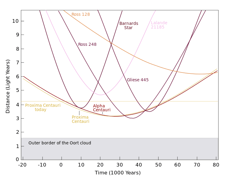
I know what you’re thinking… what about the closest? At magnitude +11, Proxima Centauri in the Alpha Centauri triple star system 4.7 light years distant didn’t quite make the cut. Barnard’s Star (see below) is the closest in this regard. Interestingly, the brown dwarf pair Luhman 16 was discovered just last year at 6.6 light years distant.

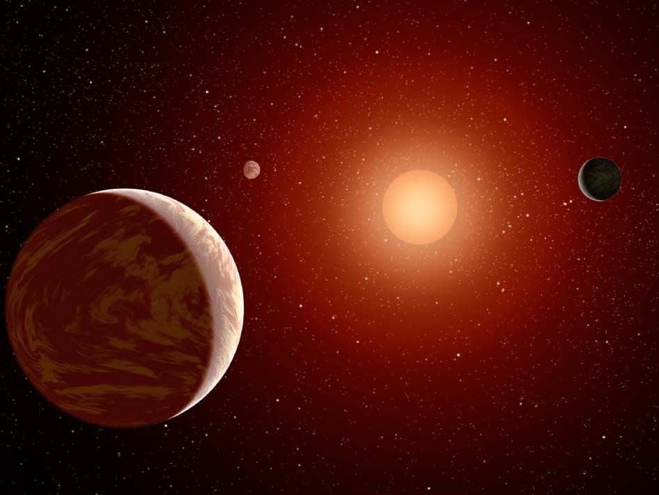
Also, do not confuse red dwarfs with massive carbon stars. In fact, red dwarfs actually appear to have more of an orange hue visually! Still, with the wealth of artist’s conceptions (see above) out there, we’re probably stuck with the idea of crimson looking red dwarf stars for some time to come.

Star	Magnitude	Constellation	R.A.	Dec
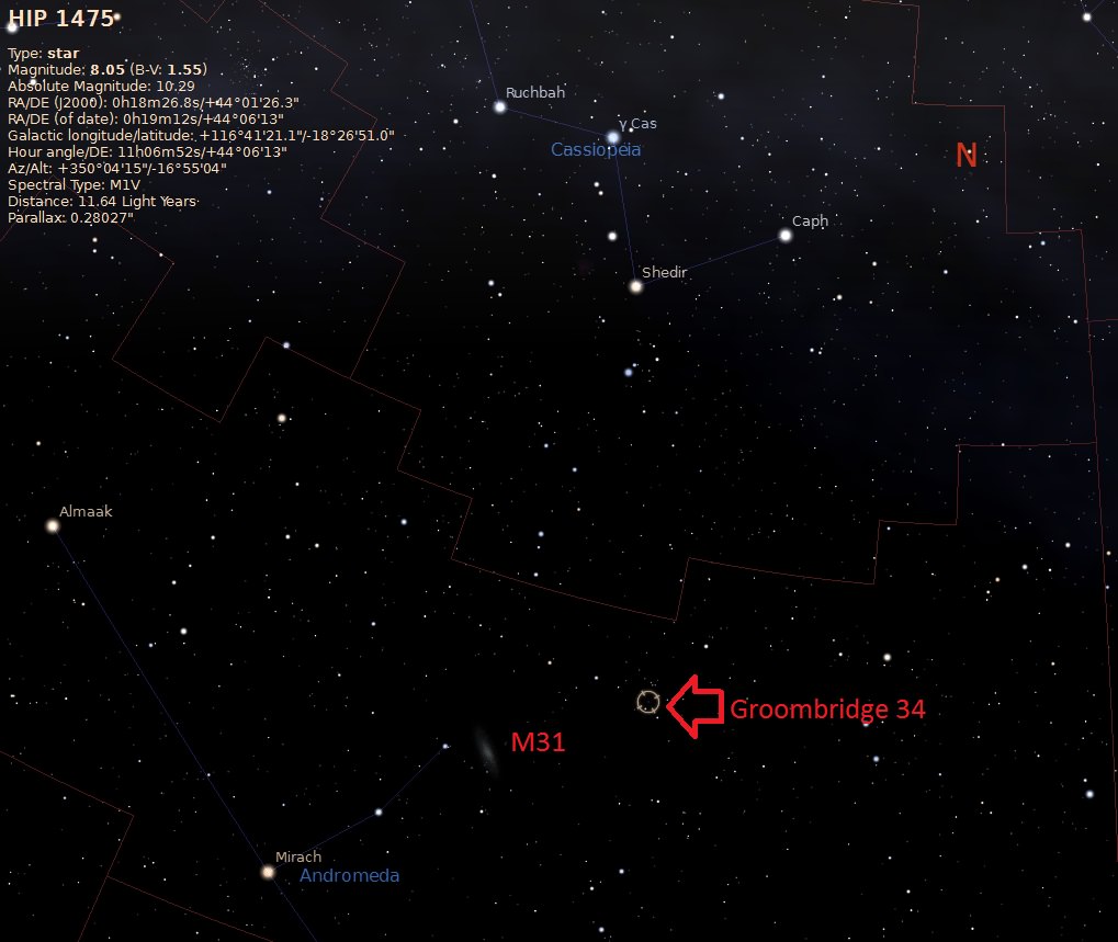
Groombridge 34	+8/11(v)	Andromeda	00h 18’	+44 01’
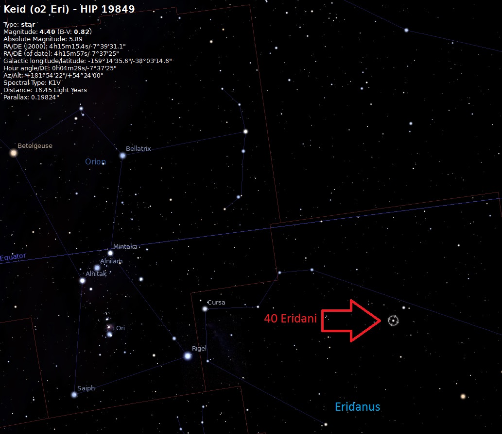
40 Eridani C	+11	Eridanus	04h 15’	-07 39’
AX Microscopii/Lacaille 8760	+6.7	Microscopium	21h 17’	-38 52’
Barnard’s Star	+9.5	Ophiuchus	17h 58’	+04 42’
Kapteyn’s Star	+8.9	Pictor	05h 12’	-45 01’
Lalande 21185	+7.5	Ursa Major	11h 03’	+35 58’
Lacaille 9352	+7.3	Piscis Austrinus	23h 06’	-35 51’
Struve 2398	+9.0	Draco	18h 43’	+59 37’
Luyten’s Star	+9.9	Canis Minor	07h 27’	+05 14’
Gliese 687	+9.2	Draco	17h 36’	+68 20’
Gliese 674	+9.9	Ara	17h 29’	-46 54’
Gliese 412	+8.7	Ursa Major	11h 05’	+43 32’
AD Leonis	+9.3	Leo	10h 20’	+19 52’
Gliese 832	+8.7	Grus	21h 34’	-49 01’

Notes on each:

Groombridge 34: Located less than a degree from the +6th magnitude star 26 Andromedae in the general region of the famous galaxy M31, Groombridge 34 was discovered back in 1860 and has a large proper motion of 2.9″ arc seconds per year.

Locating Groombridge 34. Created using Stellarium.

40 Eridani C: Our sole exception to the “10^th magnitude or brighter” rule for this list, this multiple system is unique for containing a white dwarf, red dwarf and a main sequence K-type star all within range of a backyard telescope. In sci-fi mythos, 40 Eridani is also the host star for the planet Richese in Dune and the controversial location for Vulcan of Star Trek fame.

Locating 40 Eridani. Created using Stellarium.

AX Microscopii: Also known as Lacaille 8760, AX Microscopii is 12.9 light years distant and is the brightest red dwarf as seen from the Earth at just below naked eye visibility at magnitude +6.7.

A 20 year animation showing the proper motion of Barnard's Star. Credit: Steve Quirk, images in the Public Domain. — A 20 year animation showing the proper motion of Barnard’s Star. Credit: Steve Quirk, images in the Public Domain.

Barnard’s Star: the second closest star system to our solar system next to Alpha Centuari and the closest solitary red dwarf star at six light years distant, Barnard’s Star also exhibits the highest proper motion of any star at 10.3” arc seconds per year. The center of many controversial exoplanet claims in the 20^th century, it’s kind of a cosmic irony that in this era of 1790 exoplanets and counting, planets have yet to be discovered around Barnard’s Star!

Kapteyn’s Star: Discovered by Jacobus Kapteyn in 1898, this red dwarf orbits the galaxy in a retrograde motion and is the closest halo star to us at 12.76 light years distant.

Lalande 21185: currently 8.3 light years away, Lalande 21185 will pass 4.65 light years from Earth and be visible to the naked eye in just under 20,000 years.

Lacaille 9352: 10.7 light years distant, this was the first red dwarf star to have its angular diameter measured by the VLT interferometer in 2001.

Struve 2398: A binary flare star system consisting of two +9^th magnitude red dwarfs orbiting each other 56 astronomical units apart and 11.5 light years distant.

Luyten’s Star: 12.36 light years distant, this star is only 1.2 light years from the bright star Procyon, which would appear brighter than Venus for any planet orbiting Luyten’s Star.

Gliese 687: 15 light years distant, Gliese 687 is known to have a Neptune-mass planet in a 38 day orbit.

Gliese 674: Located 15 light years distant, ESO’s HARPS spectrograph detected a companion 12 times the mass of Jupiter that is either a high mass exoplanet or a low mass brown dwarf.

Gliese 412: 16 light years distant, this system also contains a +15^th magnitude secondary companion 190 Astronomical Units from its primary.

AD Leonis: A variable flare star in the constellation Leo about 16 light years distant.

Gliese 832: Located 16 light years distant, this star is known to have a 0.6x Jupiter mass exoplanet in a 3,416 day orbit.

The closest stars to our solar system over the next 80,000 years. Credit: FrancescoA under a Creative Commons Attribution Share-Alike 3.0 Unported license.

Consider this list a teaser, a telescopic appetizer for a curious class of often overlooked objects. Don’t see you fave on the list? Want to see more on individual objects, or similar lists of quasars, white dwarfs, etc in the range of backyard telescopes in the future? Let us know. And while it’s true that such stars may not have a splashy appearance in the eyepiece, part of the fun comes from knowing what you’re seeing. Some of these stars have a relatively high proper motion, and it would be an interesting challenge for a backyard astrophotographer to build an animation of this over a period of years. Hey, I’m just throwing that out project out there, we’ve got lots more in the files…

May 12, 2014December 23, 2015 by David Dickinson

NASA West Antarctic Ice Sheet Findings: Glacier Loss Appears Unstoppable

It’s a key piece of the climate change puzzle. For years, researchers have been eyeing the stability of the Western Antarctic Ice Sheet as global temperatures rise. Melting of the ice sheet could have dire consequences for sea level rise.

And though not unexpected, news from today’s NASA press conference delivered by Tom Wagner, a cryosphere program scientist with the Earth Science Division of NASA’s Science Mission Directorate in Washington D.C., Sridhar Anandakrishnan, a professor of geosciences at Pennsylvania University, and Eric Rignot, JPL glaciologist and professor of Earth system science at the University of California Irvine was certainly troubling.

The Western Antarctic Ice Sheet is a marine-based ice sheet below sea level that is bounded by the Ronne and Ross Ice Shelf and contains glaciers that drain into the Amundsen Sea. The study announced today incorporates 40 years of data citing multiple lines of observational evidence measuring movement and thickness of Antarctic ice sheets. A key factor to this loss is a thinning along the grounding line of the glaciers from underneath. The grounding line for an ice sheet is the crucial boundary where ice becomes detached from ground underneath and stretches out to become free floating. A slow degradation of the Western Antarctic Ice Sheet has been observed, one that can be attributed to increased stratospheric circulation along with the advection of ocean heat coupled with anthropogenic global warming.

A closeup of the region: red indicates regions where flow speeds have accelerated in the past 40 years. Credit: Eric Rignot

“This sector will be a major contributor to sea level rise in the decades and centuries to come,” Rignot said in today’s press release. “A conservative estimate is it would take several centuries for all of the ice to flow into the sea.”

Thickness contributes to the driving stress of a glacier. Accelerating flow speeds stretch these glaciers out, reducing their weight and lifting them off of the bedrock below in a continuous feedback process.

A key concern for years has been the possible collapse of western Antarctica’s glaciers, leading to a drastic acceleration in sea-level rise worldwide. Such a catastrophic glacial retreat would dump millions of tons of ice into the sea over a relatively short span of time. And while it’s true that ice calves off of the Western Antarctic ice sheet every summer, the annual overall rate is increasing.

The study is backed up by satellite, airborne and ground observations looking at thickness of ice layers over decades.

Researchers stated that the Amundsen Sea Embayment sector alone contains enough ice to increase global sea level by 1.2 metres. A strengthening of wind circulation around the South Pole region since the 1980s has accelerated this process, along with the loss of ozone. This circulation also makes the process more complex than similar types of ice loss seen in Greenland in the Arctic.

The research paper, titled Widespread, rapid grounding line retreat of Pine Island, Thwaites, Smith and Kohler glaciers, West Antarctica from 1992 to 2011 has been accepted for publication in the American Geophysical Union’s journal Geophysical Research Letters. The American Association for the Advancement of Science will also be releasing a related study on the instability of the West Antarctic ice sheet today in the journal Science.

The most spectacular retreat referenced in the study was seen occurring at the Smith/Kohler glaciers, which migrated about 35 kilometres and became ungrounded over a 500 kilometre square region during the span of 1992 to 2011.

Another telling factor cited in the study was the large scale synchronous ungrounding of several glaciers, suggesting a common trigger mechanism — such as ocean heat flux — is at play.

On the ice shelf proper, the key points that anchor or pin the glaciers to the bedrock below are swiftly vanishing, further destabilizing the ice in the region.

Assets that were used in the study included interferometry data from the Earth Remote Sensing (ERS-1/2) satellites’ InSAR (Interferormetry Synthetic Aperture Radar) instruments, ground team observations and data collected from NASA’s Operation IceBridge overflights of the Antarctic. IceBridge uses a converted U.S. Navy P-3 Orion submarine hunting aircraft equipped with radar experiment packages used to take measurements of the thickness of the ice sheet.

Possible follow up studies targeting the region are upcoming, including five Earth science and observation missions scheduled to be launched this year, which include the Soil Moisture and Passive (SMAP) mission, The Orbiting Carbon Observatory (OCO-2) and the Global Precipitation Measurement (GPM) Core Observatory, launched this past February.

Along with these future NASA missions, there are also two missions — RapidScat and the Cloud-Aerosol Transport System or CATS — slated to study climate headed for the International Space Station this year.

This comes as recent United Nations and United States reports have also announced the reality of climate change and anthropogenic global warming.

“The collapse of this sector of West Antarctica appears to be unstoppable,” Rignot said. “The fact that the retreat is happening simultaneously over a large sector suggests it was triggered by a common cause, such as an increase in the amount of ocean heat beneath the floating sections of the glaciers.”

Of course, the solar cycle, volcanic activity, global dimming (via changes in reflectivity, known as albedo) and human activity all play a role in the riddle that is climate change. The bad news is, taking only natural factors into account, we should be in a cooling period right now.

And yes, reflective ice cover also plays a role in the albedo of the Earth, but researchers told Universe Today that no significant overall seasonal variations in the extent of surface layer of ice will change, as the key loss comes from the ungrounding of ice from below. Thus, this ice loss does not present a significant contribution to changes in overall global albedo, though of course, much of this additional moisture will eventually be available for circulation in the atmosphere. And the same was noted in the press conference for those pinning their hopes on the 2014 ice extent being greater than previous years, a season that was a mere blip on the overall trend. The change and retreat in the grounding line below seen in the study was irrespective of the ice extent above.

NASA’s Operation IceBridge will continue to monitor the ice flow when the next Antarctic deployment cycle resumes in October of this year.

And in the meantime, the true discussion is turning to the challenges of living with a warmer planet. Insurance companies, the Department of Defense and residents of low-lying coastal regions such as Miami’s South Beach already know that the reality of global warming and sea level rise is here. Perhaps the very fact that naysayers have at least backed up their positions a bit in recent years from “global warming isn’t happening” to “Its happening, but there are natural cycles” can at least give us a starting point for true intelligent science-based dialogue to begin.

– Social media questions from today’s conference can be reviewed at the #AskNASA hastag.

May 8, 2014December 23, 2015 by David Dickinson

Interesting Prospects for Comet A1 Siding Spring Versus the Martian Atmosphere

Inbound: the Hubble Space Telescope images Comet 2013 A1 Siding Spring with its Wide Field Camera 3. Credit: NASA.

It may be the chance of a lifetime for planetary science.

This October, a comet will brush past a planet, giving scientists a chance to study how it possibly interacts with a planetary atmosphere.

The comet is C/2013 A1 Siding Spring, and the planet in question Mars. And although an impact of the comet on the surface of the Red Planet has long been ruled out, a paper in the May 2014 issue of Icarus raises the interesting possibility of possible interactions of the coma of A1 Siding Spring and the tenuous atmosphere of Mars. The study comes out of the Department of Planetary Sciences at the University of Arizona, the Belgian Institute for Space Aeronomy, the Institut de Planétologie et d’Astrophysique de Grenoble at the Université J. Fourier in France, and the Cooperative Institute for Research in Environmental Sciences at the University of Colorado in Boulder.

For the study, researchers considered how active Comet A1 Siding Spring may be at the time of closest approach on October 19^th, 2014.

Discovered early last year by Robert McNaught from the Siding Spring Observatory in Australia, Comet A1 Siding Spring created a stir in the astronomical community when it was found that it will pass extremely close to Mars later this year. Further measurements of its orbit have since ruled this possibility out, but its passage will still be a close one, with a nominal passage of 138,000 kilometres from Mars. That’s about one third the distance from Earth to the Moon, and 17 times closer than the nearest recorded passage of a comet to the Earth, Comet D/1770 L1 Lexell in 1780. Mars’ outer moon Deimos has an orbital distance of about 23,500 kilometres.

The passage of Comet 2013 A1 Siding Spring through the inner solar system. Credit: NASA.

And although the nucleus will safely pass Mars, the brush with its extended atmosphere might just be detectable by the fleet of spacecraft and rovers in service around Mars. At a distance of 1.4 Astronomical Units (A.U.) from the Sun during the encounter, the vast coma is expected to be comprised primarily of H₂O. At an input angle of about 60 degrees, penetration was calculated in the study to impinge down and altitude of 154 kilometres to the topside of the Martian ionosphere, in the middle of the thermosphere.

Such an effect should linger for just over 4 hours, well over the interaction period of Mars’ atmosphere with the coma of just over an hour, centered on 18:30 UT on October 19^th, 2014.

What kind of views might missions like HiRISE and MSL get of the comet remains to be seen, although NEOWISE and Hubble are already monitoring the comet for enhanced activity. The Opportunity rover is also still functioning, and Mars Odyssey and ESA’s Mars Express are still in orbit around the Red Planet and sending back data. But perhaps the most interesting possibilities for observations of the event are still en route: India’s Mars Orbiter Mission and NASA’s MAVEN orbiter arrive just before the comet. MAVEN was designed to study the upper atmosphere of Mars, and carries an ion-neutral mass spectrometer (NGIMS) which could yield information on the interaction of the coma with the Martian upper atmosphere and ionosphere. The NGIMS cover is slated for release just two days before the comet encounter. All spacecraft orbiting Mars may feel the increased drag effects of the encounter.

A simulation of Mars as seen from Comet A1 Siding Spring on closest approach. Created by the author using Starry Night Software.

Proposals for using Earth-based assets for further observations of the comet prior to the event in October are still pending. Amateur observers will be able to follow the approach telescopically, as Comet A1 Siding Spring is expected to reach +8^th magnitude in October and pass 7’ from Mars in the constellation Ophiuchus as seen from the Earth. Mars just passed opposition last month, but both will be low to the south west at dusk for northern hemisphere observers in October.

It’s also interesting to consider the potential for interactions of the coma with the surfaces of the moons of Mars as well, though the net amount of water vapor expected to be deposited will not be large.

UPDATE: Check out this nifty interactive simulator which includes Comet A1 Siding Springs courtesy of the Solar System Scope:

The H₂O coma of A1 Siding Spring is expected to have a radius of 150,000 kilometres when it passes Mars, just a shade over the nominal flyby distance.

“There is a more extended coma made up of H₂O dissociation products (such as hydrogen and hydroxide) that extends for ~1,000,000 kilometres,” researcher at the Department of Planetary Sciences at the University of Arizona and lead author on the paper Roger Yelle told Universe Today.

“Essentially, Mars is in the outer reaches of the coma. The main ion tail misses Mars but there will be some ions from the comet that do reach Mars. The dust tail just misses Mars, which is fortunate.”

The paper also notes that significant perturbations of the upper atmosphere of Mars will occur if the cometary production rate is 10^28 s-1 or larger, which corresponds to about 300 kilograms per second.

“The MAVEN spacecraft will make very interesting observations,” Roger Yelle also told Universe Today. “The comet will perturb primarily the upper atmosphere of Mars and MAVEN was designed to study the upper atmosphere of Mars. Also, it’s just such an incredible coincidence that the comet arrives at Mars less than one month after MAVEN does. MAVEN is nominally in its checkout phase then, and the main science phase of the mission was not scheduled to start until November 1^st. However, we are reassessing our plans to see what observations we can make. It’s all quite exciting, and we have to balance safety and the desire to make the best science measurements.”

It’s an unprecedented opportunity, that’s for sure… all eyes will be on the planet Mars and Comet A1 Siding Spring on October the 19^th!

May 7, 2014December 23, 2015 by David Dickinson

The Hunt for KBOs for New Horizons’ Post-Pluto Encounter Continues

An artist’s conception of a KBO encounter by New Horizons. Credit: JHUAPL/SwRI.

Are you ready for the summer of 2015? A showdown of epic proportions is in the making, as NASA’s New Horizons spacecraft is set to pass within 12,500 kilometres of Pluto — roughly a third of the distance of the ring of geosynchronous satellites orbiting the Earth — a little over a year from now on July 14th, 2015.

But another question is already being raised, one that’s assuming center stage even before we explore Pluto and its retinue of moons: will New Horizons have another target available to study for its post-Pluto encounter out in the Kuiper Belt? Researchers say time is of the essence to find it.

To be sure, it’s a big solar system out there, and it’s not that researchers haven’t been looking. New Horizons was launched from Cape Canaveral Air Force Station on January 19^th, 2006 atop an Atlas V rocket flying in a 551 configuration in one of the fastest departures from Earth ever: it took New Horizons just nine hours to pass Earth’s moon after launch.

New Horizons spends its last days on Earth pre-encapsulation. (Credit: NASA/KSC).

The idea has always been out there to send New Horizons onward to explore and object beyond Pluto in the Kuiper Belt, but thus far, searches for a potential target have turned up naught.

A recent joint statement from NASA’s Small Bodies and Outer Planets Assessment Groups (SBAG and OPAG) has emphasized the scientific priority needed for identifying a possible Kuiper Belt Object (KBO) for the New Horizons mission post-Pluto encounter. The assessment notes that such a chance to check out a KBO up close may only come once in our lifetimes: even though it’s currently moving at a heliocentric velocity of just under 15 kilometres a second, it will have taken New Horizons almost a decade to traverse the 32 A.U. distance to Pluto.

The report also highlights the fact that KBOs are expected to dynamically different from Pluto as well and worthy of study. The statement also notes that the window may be closing to find such a favorable target after 2014, as the upcoming observational apparition of Pluto as seen from Earth — and the direction New Horizons is headed afterwards — reaches opposition this summer on July 4^th.

But time is of the essence, as it will allow researchers to plan for a burn and trajectory change for New Horizons shortly after its encounter with Pluto and Charon using what little fuel it has left. Then there’s the issue of debris in the Pluto system that may require fine-tuning its trajectory pre-encounter as well. New Horizons will begin long range operations later this year in November, switching on permanently for two years of operations pre-, during and post- encounter with Pluto.

And there currently isn’t a short-list of “next best thing” targets for New Horizons post-Pluto encounter. One object, dubbed VNH0004, may be available for distant observations in January of next year, but even this object will only pass 75 million kilometres — about 0.5 A.U. — from New Horizons at its closest.

Ground based assets such as the Keck, Subaru and Gemini observatories have been repeatedly employed in the search over the past three years. The best hopes lie with the Hubble Space Telescope, which can go deeper and spy fainter targets.

Nor could New Horizons carry out a search for new targets on its own. Its eight inch (20 cm in diameter) LORRI instrument has a limiting magnitude of about +18, which is not even close to what would be required for such a discovery.

New Horizons currently has 130 metres/sec of hydrazine fuel available to send it onwards to a possible KBO encounter, limiting its range and maneuverability into a narrow cone straight ahead of the spacecraft. This restricts the parameters for a potential encounter to 0.35 A.U. off of its nominal path for a target candidate be to still be viable objective. New Horizons will exit the Kuiper Belt at around 55 A.U. from the Sun, and will probably end its days joining the Voyager missions probing the outer solar system environment. Like Pioneers 10 and 11, Voyagers 1 and 2 and the upper stage boosters that deployed them, New Horizons will escape our solar system and orbit the Milky Way galaxy for millions of years. We recently proposed a fun thought experiment concerning just how much extraterrestrial “space junk” might be out there, littering the galactic disk.

And while the crowd-sourced Ice Hunters project generated lots of public engagement, a suitable target wasn’t found. There is talk of a follow up Ice Investigators project, though it’s still in the pending stages.

Another issue compounding the problem is the fact that Pluto is currently crossing the star rich region of the Milky Way in the constellation Sagittarius. Telescopes looking in this direction must contend with the thousands of background stars nestled towards the galactic center, making the detection of a faint moving KBO difficult. Still, if any telescope is up to the task, it’s Hubble, which just entered its 25^th year of operations last month.

Credit Starry Night — The path of Pluto through the constellation Sagittarius through August 2015. Credit: Starry Night.

Shining at +14^th magnitude, Pluto will be very near the 3.5^th magnitude star Xi² Sagittarii during the July 2015 encounter.

New Horizons is currently 1.5 degrees from Pluto — about 3 times the angular size of a Full Moon —as seen from our Earthly vantage point, and although neither can be seen with the naked eye, you can wave in their general direction this month on May 18^th, using the nearby daytime Moon as a guide.

July 2015 will be an exciting and historic time in solar system exploration. Does Pluto have more undiscovered moons? A ring system of its own? Does it resemble Neptune’s moon Triton, or will it turn out looking entirely different ?

If nothing else, exploration of Pluto will finally give us science writers some new images to illustrate articles on the distant world, rather than recycling the half a dozen-odd photos and artist’s conceptions that are currently available. An abundance of surface features will then require naming as well. It would be great to see Pluto’s discoverer Clyde Tombaugh and Venetia Burney — the girl who named Pluto — get their due. We’ll even assume our space pundit’s hat and predict a resurgence of the “is it a planet?” debate once again in the coming year as the encounter nears…

Onward to Pluto and the brave new worlds beyond!

May 5, 2014December 23, 2015 by David Dickinson

Comet Jacques Brightens: How to See it in May

Comet Jacques as imaged on March 18th, shortly after discovery. Credit: Efrain Morales Rivera.

A recently discovered comet is headed northward and is set to put on one of two fine performances for binocular observers in 2014 starting this week.

Comet C/2014 E2 Jacques was discovered on March 13^th 2014 by Cristóvão Jacques, Eduardo Pimentel and João Ribeiro de Barros while observing from the Southern Observatory for Near Earth Asteroids Research (SONEAR) facility located near Oliveira, Brazil.

The comet was just about at +15^th magnitude at the time of discovery as it glided across the southern hemisphere constellation of Centaurus.

While a majority of comet discoveries are destined to remain small and faint, Comet Jacques was immediately shown to be something special. Upon discovery of any new comet, the first task is to gain several observations hours or nights apart to accurately gauge its distance and orbit. Are astronomers looking at a small, garden variety comet close up, or a large, active one far away?

In the case of Comet Jacques, it was something in between: a comet about 1.22 Astronomical Units (A.U.s) distant at time of discovery. Comet Jacques is headed towards perihelion 0.66 A.U. from the Sun in early July and will pass 0.56 A.U. from Earth on August 28th. Follow up observations carried out using the iTelescope at Siding Spring Australia showed a slightly elongated coma about 2 arc minutes across shortly after discovery, and the comet has recently jumped up to magnitude +8 — ahead of the projected light curve — in just the past week.

The path of Comet Jacques, looking west from latitude 30 degree north 45 minutes after sunset. Credit: Starry Night.

We caught our first good look at Comet Jacques last night while setting up for the Virtual Star Party. While +10 magnitude or brighter is usually a pretty good rule of thumb for binocular visibility, we found that the comet was only apparent as a fuzzy smudge viewing it with a 8” Schmidt-Cassegrain telescope using averted vision at low power. Remember, the brightness of a comet is spread out over its apparent surface area, similar to viewing a diffuse nebula. Our first telescopic views of the ill-fated comet ISON as it breeched +10^th magnitude were similar. Certainly, a nearby waxing crescent Moon in Gemini last night didn’t help.

How bright will Comet Jacques get? Current projections call for it to perhaps break naked eye visibility around +6^th magnitude after June 1^st and reach as bright as +4^th magnitude in early July near perihelion. After its first evening act in May and June, Comet Jacques will reemerge in the dawn sky for northern hemisphere observers for Act 2 and trace a path northward paralleling the galactic plane through the star rich fields of Perseus, Cassiopeia, Cepheus and Cygnus in August and September of this year. If our luck holds out, Comet Jacques will remain above 6^th magnitude until early September.

Credit JPL — The path of Comet Jacques through the inner solar system. Credit: JPL solar system small body generator.

This comet also created a brief flurry of interest when it was revealed that it will pass just 0.085 AUs or 12,700,000 kilometers from Venus on July 13^th, 2014. Though close, this is still 31 times the distance from Earth to the Moon. The only “eyes” that humanity has currently in operation around Venus is ESA’s Venus Express orbiter. During closest approach Comet Jacques will appear just over 3 degrees away from Venus as seen from our Earthly vantage point.

Another comet is also set to photobomb a planet, as Comet A1 Siding Spring passes a nominal distance of 0.0009 A.U.s or 135,000 kilometers from Mars this Fall on October 19th.

The closest recorded passage of a comet near Earth was Comet D/1770 L1 Lexell in 1770, which passed us 0.015 A.U.s or 233 million kilometres distant.

Now on to Act 1. May finds Comet Jacques spending most of the month in the long rambling constellation of Monoceros. Currently moving just under 2 degrees a day, Comet Jacques crosses the celestial equator northward this week on May 8^th. You’ll note its high orbital inclination of 156.4 degrees as it speeds northward. Comet Jacques has a long orbital period gauged at over 30,000 years — the last time Comet Jacques visited the inner solar system, our ancestors had the Last Glacial Maximum period to look forward to.

Light curve — The projected light curve of comet Jacques with recent observations. Credit: Seiichi Yoshida/aerith.net.

Comet Jacques is currently the brightest comet “with a bullet,” edging out the +9^th magnitude comets C/2012 K1 PanSTARRS gilding through Canes Venatici and comet C/2012 X1 LINEAR, currently residing in the constellation of Aquila the Eagle. A great place to keep up with current observations of comets is the Comet Observation Database. We’re also pinging the IAU Minor Planet Center’s quick look page for new discoveries daily.

Here are some highlights to watch out for as Comet Jacques heads towards perihelion. Passages within one degree — twice the size of the Full Moon — near stars brighter than +5^th magnitude are noted unless mentioned otherwise:

The celestial path of Comet Jacques from May 3rd through June 1st. Credit: Starry Night.

May 8^th: Passes the +4.1 magnitude star Delta Monocerotis and crosses north of the celestial equator.

May 10^th: Passes planetary nebula NGC 2346.

May 11^th: Passes briefly into Canis Minor before reentering the constellation Monoceros.

May 14^th: Full Moon occurs, marking the start of a favorable two week period of moonless evenings soon after.

May 24^th: Passes the +4.8 magnitude star 17 Monocerotis.

May 28^th: New Moon occurs, marking the return of the Moon to early evening skies.

May 29^th: Passes the +4.7 magnitude star 15 Monocerotis.

May 30^th: Passes the Christmas tree cluster. Photo op!

May 31^st: The waxing crescent Moon passes less than 8 degrees from Comet Jacques.

June 1^st: Comet Jacques reaches naked eye visibility?

June 6^th: Crosses into the constellation Gemini.

June 11^th: Crosses into the constellation Taurus.

June 13^th: Full Moon occurs.

June 14^th:Crosses the galactic plane.

June 21^st: Passes into the field of view of SOHO’s LASCO C3 camera.

June 27^th: New Moon occurs.

July 2^nd: Reaches perihelion at 0.6638 A.U. from the Sun.

July 8^th: Crosses north of the ecliptic plane.

July 13^th: Passes 0.085 A.U. from Venus.

August 28^th: Passes 0.56 A.U. from Earth.

And thus, Comet Jacques joins the parade of fine binocular comets in the 2014 night sky, as the stage is set for Act 2 this fall. And keep in mind, the next “big one” could grace our skies at anytime… more to come!

April 29, 2014December 23, 2015 by David Dickinson

Amazing Images of Today’s Solar Eclipse from Earth and Space

The images are pouring in. While most of North America slept this AM, Australians were treated to the very first solar eclipse of 2014 earlier today. And while this particular eclipse was a partial one only from the Australian continent, it still offered observers a fine view of an often elusive natural spectacle.

The partial eclipse as seen from Adelaide. Credit: Michael Drew (@MichaelDrew1234)

Although rain and clouds frustrated attempts to view the eclipse from much of southern Australia, clouds parted long enough in Queensland to the east and areas around Perth to the west to offer observers a fine view. Many eclipse watchers on the Australian east coast had the additional bonus of catching the setting Sun during the eclipse.

A quick screen shot from ESA’s Proba-2 spacecraft during one of the three passes of the solar eclipse. Credit: ESA/Proba-2.

We wrote about the prospects for catching this bizarre eclipse previously. The eclipse was a rare, non-central annular with one limit only, meaning the antumbra or inner core of the Moon’s shadow just grazed the edge of the planet over Antarctica. We haven’t yet heard if anyone witnessed it from the southern polar continent, though two year round research stations were located near the path of annularity. The European Space Agency operates Concordia Station nearby as part of its Human Spaceflight Activities program and they were aware of the upcoming event. We’ll keep you updated if reports or images surface!

The eclipse seen through clouds. Photographer David Herne also noted that while he used his D3100 DSLR for the shot, his homemade pinhole camera offered fine views as well! Credit: David Herne(@AunaEridu)/Perth Western Australia.

As predicted, another solar observing sentinel in low Earth orbit did indeed witness the eclipse. ESA’s Proba-2 spacecraft caught the eclipse on three passes in this amazing raw animation from its SWAP-2 camera. The final third pass goes by extremely quick –these are measured in minutes from Proba-2’s swift vantage point – but the Sun looks well nigh to greater than 95% eclipsed by the Moon as it flies by.

The partial solar eclipse as seen from Adelaide, Australia. Credit: Silveryway.

There’s no word as of yet if the joint NASA/JAXA mission Hinode caught the eclipse as well, but we’ll keep you posted!

UPDATE: Courtesy of the European Space Agency and the Royal Observatory of Belgium, we now give you the full YouTube timelapse of the eclipse courtesy of Proba-2:

You’ll note that Proba-2 caught the partial phases on four separate passes… we also checked the sequence frame by frame, and although it looks like Proba-2 “may” have seen an annular – or even total – eclipse from space, it looks like it did so between captures!

This eclipse is one of two solar eclipses and four eclipses total for 2014. An interesting discussion occurred leading up to this eclipse as to the minimum number of eclipses that can occur in a year, which is four. If, however, you exclude faint lunar penumbrals, that number does indeed drop to two, both of which must be solar, which occurs in 2016. This also sparked a lively debate as to the naming of such a year on Twitter, with everything from a “Dwarf Eclipse Year” to “Nano Eclipse Cycle” and “Spurious Eclipse Year” being proposed. We liked the suitably esoteric and ready tweet-able term “declipsy” ourselves… thanks for the proposals and the lively discussion!

The partially-eclipsed Sun sinks into the west as seen from Brisbane, Australia on April 29, 2014. Credit and copyright: Teale Britstra.

Partial solar eclipse in Adelaide, South Australia on April 29, 2014. Credit and copyright: Silveryway on Flickr.

Thanks also to all who sent in pics. We’ll be updating this post as more come in… and although eclipse season 1 of 2 may be over for now, 2014 still has another total lunar eclipse and a good partial solar in October, both visible from North America.

…And we’re only three years out and have just two more total solar eclipses to go until the historic total solar eclipse of August 21^st, 2017…

Let the countdown begin!

UPDATE: Missed out on the solar eclipse today? Hey so did we, it happens to the best of us… luckily, YOU can now relive the all of the excitement of the eclipse courtesy of the folks from the Virtual Telescope Project in YouTube Splendor:

And finally: got pics of the partial solar eclipse that you took today and you want to share with the world? Put ’em up on Universe Today’s Flickr community and let us know!

April 23, 2014December 23, 2015 by David Dickinson

Saturn at Opposition: Our 2014 Guide

Saturn as imaged from Aguadilla, Puerto Rico on April 15th. Credit: Efrain Morales.

Planet lovers can rejoice: one of the finest jewels of the solar system in returning to the evening night sky.

The planet Saturn reaches opposition next month on May 10^th. This means that as the Sun sets to the west, Saturn will rise “opposite” to it in the east, remaining well positioned for observation in the early evening hours throughout the summer season. In fact, we’ll have four of the five naked eye planets above the horizon at once for our evening viewing pleasure in the month of May, as Jupiter also rides high to the west at sunset, Mars just passed opposition last month and Mercury reaches greatest eastern elongation on May 25^th. Venus is the solitary holdout, spending a majority of 2014 in the dawn sky.

Saturn will shine at magnitude +0.3 this month and its disk spans an apparent 19,” or 44” if you take into account the apparent width of its rings. The rings are currently tipped open 22 degrees with respect to our line of sight. The ring opening is widening, and will reach a maximum of over 25 degrees in 2017 before the trend reverses. Anyone who remembers observing Saturn back in 2009 will recall that its rings were edge on to our view. This widening of Saturn’s rings also lends itself to a curious effect: although we’re in a cycle of oppositions that are getting farther away — Saturn is 12.5 million kilometres or 0.083 Astronomical Units (A.U.s) more distant in 2014 than it was during opposition last year as it’s headed towards aphelion in 2018 — its widening rings are actually making it appear a bit brighter.

The path of Saturn through the constellation Libra from April through October 2014. Created using Starry Night Education Software.

This year’s opposition will find Saturn in the astronomical constellation of Libra, where it’ll spend most of 2014. Oppositions of the ringed planet are set to continue to “head south” until 2018, and won’t occur north of the celestial equator again until 2026. I remember when oppositions of Saturn returned to the constellation Virgo a few years back — where I had first looked at it with my 60mm Jason refractor as a teenager — and realizing that I had now been into observational astronomy for roughly one “Saturnian year.”

The ancients had little knowledge of how unique Saturn was. The faintest and slowest moving of the classical planets, even Galileo knew that something was up when he turned his first primitive telescope towards it. His sketches depict Saturn as something similar to a double handled coffee cup, a testament to how poor his view really was. It wouldn’t be until Christiaan Huygens in 1655 that the true nature of Saturn’s rings was deduced as a flat and separate feature from the disk.

At opposition, the disk of the planet casts a shadow straight back from our point of view. This vantage slowly changes as the planet moves towards eastern quadrature on August 9th and we get a glimpse slightly off to one side of the planet. After opposition, the shadow of the disk can again be seen casting back onto the rings.

An outstanding IPhone 4S capture of Saturn on April 20th, 2014. Credit: Andrew Symes, @FailedProtostar.

Another interesting phenomenon to watch out for near opposition is known as the Seeliger effect. Also sometimes referred to as the “opposition surge,” this sudden brightening of the disk and rings is a subtle effect, as the globe of Saturn and all of those tiny little ice crystals reach 100% illumination. This effect can be noted to the naked eye on successive nights around opposition, and will get more prominent towards 2017. Coherent-backscattering of light has also been proposed as a possible explanation of this phenomenon. Perhaps a video sequence capturing this effect is in order for skilled astro-imagers in 2014.

Through a small telescope, the first feature that becomes apparent is Saturn’s glorious system of rings. Crank up the magnification, and you’ll note a dark groove in the ring system. This is the Cassini Division, first described by Giovanni Cassini in 1675.

Here’s a challenge we came across some years back: can you see the disk of Saturn through the Cassini Division? Right around opposition is a good time to attempt this unusual feat of visual athletics.

A sample simulation depicting the orientation of Saturn's observable moons on the night of May 9th. Created using Starry Night Education software. — A sample simulation depicting the orientation of Saturn’s observable moons on the night of May 9th. Created using Starry Night Education software.

Saturn’s large moon Titan is an easy catch at magnitude +8 in a small telescope. Titan is the second largest moon in the solar system. Place it in a direct orbit about the Sun, and it would be considered a planet, no problem. 7 of Saturn’s 62 known moons are within reach of a small telescope. In addition to Titan, they are, with quoted magnitudes: Mimas (+13), Enceladus (+12), Tethys (+10), Rhea (+10), Dione (+11) and Iapetus. Iapetus is of special interest, as it brightens from +11.9 to magnitude +10.2 as it traces out its 79 day orbit. We always knew there was something unique about this moon, and NASA’s Cassini mission revealed the world to have two distinctly different hemispheres with vastly different albedos during its close 2007 flyby.

The close passage of the Full Moon near Saturn on May 14th. Created using Stellarium.

Also, be sure to check out Saturn on the night of May 14^th — just 4 nights after opposition — as the Full Moon sits less than a degree south of the ringed planet. Can you see both in the same telescopic field of view? Can you nab Saturn next to the rising daytime Moon low to the horizon just before local sunset? The Moon will actually occult (pass in front of) Saturn for viewers based in Australia and New Zealand on the 14^th. This is only one of 11 occultations — nearly one for each lunation — of Saturn by the Moon in 2014. Unfortunately, the best one for North America occurs in the daytime on August 31^st, though it too may be observable telescopically.

The foot print of the May 14th occultation of Saturn by the Moon. Credit: Occult 4.0. — The footprint of the May 14th occultation of Saturn by the Moon. Credit: Occult 4.0.

Finally, this evening apparition of the planet runs through northern hemisphere summer and fall until Saturn reaches solar conjunction on November 18th. So get those homemade planetcams out, send those pics in to Universe Today, and be sure to join in to the Virtual Star Party every Sunday Night… Saturn is sure to be featured!

April 22, 2014April 26, 2016 by David Dickinson

Remembering John Houbolt: the Man Who Gave Us Lunar Orbit Rendezvous

John Houbolt demonstrating Lunar Orbit Rendezvous circa 1962. Credit: NASA.

The space community lost a colossus of the of the Apollo era last week, when John Houbolt passed away last Tuesday just five days after his 95^th birthday.

Perhaps the name isn’t as familiar to many as Armstrong or Von Braun, but John Houbolt was a pivotal figure in getting us to the Moon.

Born in Altoona, Iowa on April 10^th, 1919, Houbolt spent most of his youth in Joliet, Illinois. He earned a Masters degree in Civil Engineering from the University of Illinois at Urbana-Champaign in 1942 and a PhD in Technical Sciences from ETH Zurich in Switzerland in 1957. But before that, he would become a member of the National Advisory Committee for Aeronautics (NACA) in 1942, an organization that would later become the National Aeronautics and Space Administration or NASA in 1958.

It was 1961 when Houbolt made what would be his most enduring mark on the space program. He was working as an engineer at the Langley Research Center, at a time when NASA and the United States seriously needed a win in the space race. The U.S.S.R. had enjoyed a long string of firsts, including first satellite in orbit (Sputnik 1, October 1957), first spacecraft to photograph the lunar farside (Luna 3 in October 1959) and first human in space with the launch of Yuri Gagarin aboard Vostok 1 in April 1961. A young President Kennedy would make his now famous “We choose to go to the Moon…” speech at Rice University later the next year in late 1962. Keep in mind, in U.S. astronaut John Glenn had just made his first orbital flight months before Kennedy’s speech, and total accumulated human time in space could be measured in mere hours. Unmanned Ranger spacecraft were having a tough time even getting off of the pad, and managing to crash a space probe into the Moon was considered to be a “success”. The task of sending humans “by the end of this decade” was a daunting one indeed…

NASA would soon have a mandate to sent humans to the Moon: but how could they pull it off?

Early ideas for manned lunar missions envisioned a single gigantic rocket that would head to the Moon and land, Buck Rodgers style, “fins first.” Such a rocket would have to be enormous, and carry the fuel to escape Earth’s gravity well, land and launch from the Moon, and return to Earth.

A second approach, known as Earth-orbit rendezvous, would see several launches assemble a mission in low Earth orbit and then head to the Moon. Curiously, though this was an early idea, it was never used in Apollo, though it was briefly resurrected during the now defunct Constellation Program.

But it was a third option that intrigued Houbolt, known as Lunar Orbit Rendezvous. LOR had been proposed by rocket pioneers Yuri Kondratyuk and Hermann Oberth in 1923, but had never been seriously considered. It called for astronauts to depart the Earth in a large rocket, and instead, use a small lander designed only to land and launch from the Moon while the spacecraft for Earth return orbited overhead.

Houbolt became a staunch advocate for the idea, and spent over a year convincing NASA officials. In one famous letter to NASA associate administrator Robert Seamans, Houbolt was known to have remarked “Do we want to go to the Moon or not?”

It’s interesting to note that it was probably only in a young organization like the NASA of the early 1960s that, in Houbolt’s own words, a “voice in in the wilderness” could be heard. Had NASA become a military run organization — as many advocated for in the 1950s — a rigid chain of command could have meant that such brash ideas as Houbolt’s would have never seen the light of day. Thank scientists such as James Van Allen for promoting the idea of a civilian space program that we take for granted today.

Even then, selling LOR wasn’t easy. The idea looked preposterous: astronauts would have to learn how to undock and dock while orbiting a distant world, with no chance of rescue. There was no second chance, no backup option. Early plans called for an EVA for astronauts to enter the Lunar Module prior to descent which were later scrapped in favor of extracting it from atop the third stage and boarding internally before reaching the Moon.

Once Houbolt had sold key visionaries such as Wernher von Braun on the idea in late 1962, LOR became the way we would go to the Moon. And although Houbolt’s estimations of the mass required for the Lunar Module were off by a factor of three, the story is now the stuff of early Apollo era legend. You can see Houbolt (played by Reed Birney) and the tale of the LM and LOR in the From Earth to the Moon episode 5 entitled “Spider”.

Houbolt was awarded NASA’s medal for Exceptional Scientific Achievement in 1963, and he was in Mission Control When Apollo 11 touched down in the Sea of Tranquility.

He passed away in a Scarborough, Maine nursing home last Tuesday, and joins other unsung visionaries of the early space program such as Mary Sherman Morgan. It’s sad to think that we may soon live in a world where those who not only walked on the Moon, but those who also sent us and knew how to get there, are no longer with us.

Thanks, John… you gave us the Moon.

April 21, 2014December 23, 2015 by David Dickinson

Our Guide to the Bizarre April 29th Solar Eclipse

The 2013 partial eclipse rising over the Vehicle Assembly Building along the Florida Space Coast. This month's solar eclipse will offer comparable sunset views for eastern Australia. Photo by author.

Will anyone see next week’s solar eclipse? On April 29^th, an annular solar eclipse occurs over a small D-shaped 500 kilometre wide region of Antarctica. This will be the second eclipse for 2014 — the first was the April 15^th total lunar eclipse — and the first solar eclipse of the year, marking the end of the first eclipse season. 2014 has the minimum number of eclipses possible in one year, with four: two partial solars and two total lunars. This month’s solar eclipse is also a rarity in that it’s a non-central eclipse with one limit. That is, the center of the Moon’s shadow — known as the antumbra during an annular eclipse — will juuuust miss the Earth and instead pass scant kilometres above the Antarctic continent.

The "footprint" of the April 29th solar eclipse. Credit: — The “footprint” of the April 29th solar eclipse. Credit: Eclipse predictions by Fred Espenak, NASA/GSFC.

A solar eclipse is termed “non-central with one limit” when the center of the Moon’s umbra or antumbra just misses the Earth and grazes it on one edge. Jean Meeus and Fred Espenak note that out of 3,956 annular eclipses occurring from 2000 BCE to 3000 AD, only 68 (1.7%) are of the non-central variety. An annular eclipse occurs when the Moon is too distant to cover the disk of the Sun, resulting in a bright “annulus” or “ring-of-fire” eclipse. A fine example of just such an eclipse occurred over Australia last year on May 10^th, 2013. An annular eclipse crossed the United States on May 10^th, 1994 and will next be seen from the continental U.S. on October 14^th 2023. But of course, we’ll see an end the “total solar eclipse drought” long before that, when a total solar eclipse crosses the U.S. on August 21^st, 2017!

An animated .gif of the April 29th eclipse. Credit: NASA/GSFC/A.T. Sinclair.

The “centrality” of a solar eclipse or how close a solar eclipse comes to crossing the central disk of the Earth is defined as its “gamma,” with 0 being a central eclipse, and 1 as the center of the Moon’s shadow passing 1 Earth radii away from central. All exclusively partial eclipses have a gamma greater than 1. The April 29^th eclipse is also unique in that its gamma is very nearly 1.000… in fact, combing the 5,000 year catalog of eclipses reveals that no solar eclipse from a period of 2000 B.C. to 3000 A.D. comes closer to this value. The solar eclipses of October 3^rd, 2043 and March 18^th, 1950 are, however very similar in their geometry. Guy Ottewell notes in his 2014 Astronomical Calendar that the eclipses of August 29^th, 1486 and January 8^th, 2141 also come close to a gamma of 1.000. On the other end of the scale, the solar eclipse of July 11^th 1991 had a gamma of nearly zero. This eclipse is part of saros series 148 and is member 21 of 75. This series began in 1653 and plays out until 2987 AD. This saros will also produce one more annular eclipse on May 9^th 2032 before transitioning to a hybrid and then producing its first total solar eclipse on May 31^st, 2068. But enough eclipse-geekery. Do not despair, as several southern Indian Ocean islands and all of Australia will still witness a fine partial solar eclipse from this event. Antarctica has the best circumstances as the Sun brushes the horizon, but again, the tiny sliver of “annularity” touches down over an uninhabited area between the Dumont d’Urville and Concordia stations currently occupied by France… and it just misses both! And remember, its astronomical fall headed towards winter “down under,” another strike against anyone witnessing it from the polar continent. A scattering of islands in the southern Indian Ocean will see a 55% eclipsed Sun. Circumstances for Australia are slightly better, with Perth seeing a 55% eclipsed Sun and Sydney seeing a 50% partial eclipse.

The view of the eclipse from multiple locations across the Australian continent at 7:00 UT on April 29th. Created by the author using Stellarium.

Darwin, Bali Indonesia and surrounding islands will see the Moon just nick the Sun and take a less than 20% “bite” out of it. Observers in Sydney and eastern Australia also take note: the eclipse occurs low to the horizon to the west at sunset, and will offer photographers the opportunity to grab the eclipse with foreground objects. Viewing a partial solar eclipse requires proper eye protection throughout all phases. The safest method to view a partial solar eclipse is via projection, and this can be done using a telescope (note that Schmidt-Cassegrain scopes are bad choice for this method, as they can heat up quickly!) or nothing more sophisticated than a spaghetti strainer to create hundreds of little “pinhole projectors.”

A simulation of the view that no one will see: the annular eclipse one kilometre above latitude 71S longitude 131E above the Antarctic. Created using Stellarium. — A simulation of the view that no one will see: the annular eclipse as seen hovering one kilometre above the Antarctic at latitude 71S longitude 131E . Created using Stellarium.

And although no human eyes may witness the annular portion of this eclipse, some orbiting automated ones just might. We ran some simulations using updated elements, and the European Space Agency’s Sun observing Proba-2 and the joint NASA/JAXA Hinode mission might just “thread the keyhole” and will witness a brief central eclipse for a few seconds on April 29^th: And though there’ll be few webcasts of this remote eclipse, the ever-dependable Slooh is expected to carry the eclipse on April 29th. Planning an ad hoc broadcast of the eclipse? Let us know! As the eclipse draws near, we’ll be looking at the prospects for ISS transits and more. Follow us as @Astroguyz as we look at these and other possibilities and tell our usual “tales of the saros”. And although this event marks the end of eclipse season, its only one of two such spans for 2014… tune in this October, when North America will be treated to another total lunar eclipse on the 8^th and a partial solar eclipse on the 23^rd… more to come! Send in those eclipse pics to the Universe Today Flickr community… you just might find yourself featured in this space!

April 18, 2014December 23, 2015 by David Dickinson

Get Ready for the Lyrid Meteor Shower: Our Complete Guide for 2014

A composite of 33 Lyrid meteors captured by the UK Meteor Network cameras in 2012. Credit: @UKMeteorNetwork

The month of April doesn’t only see showers that bring May flowers: it also brings the first dependable meteor shower of the season. We’re talking about the Lyrid meteors, and although 2014 finds the circumstances for this meteor shower as less than favorable, there’s still good reason to get out this weekend and early next week to watch for this reliable shower.

The Lyrid meteor shower typically produces a maximum rate of 10-20 meteors per hour, although outbursts topping over a hundred per hour have been observed on occasion. The radiant, or the direction that the meteors seem to originate from, lies at right ascension 18 hours and 8 minutes and declination +32.9 degrees north. This is just about eight degrees to the southwest of the bright star Vega, which is the brightest star in the constellation of Lyra the Lyre, which also gives the Lyrids its name.

Fun fact: this radiant actually lies juuusst across the border of Lyra in the constellation of Hercules… technically, the “Lyrids” should be the “Herculids!” This is because the shower was identified and named in the 19th century before the International Astronomical Union officially adopted the modern layout we use for the constellations in 1922.

The rising Lyrid radiant, looking to the north east at 2AM local from latitude 30 degrees north. Created using Stellarium. — The rising Lyrid radiant, looking to the northeast at 2AM local from latitude 30 degrees north. Created using Stellarium.

The source of the Lyrids was tracked down in the late 1860s by mathematician Johann Gottfried Galle to Comet C/1861 G1 Thatcher, the path of which came within 0.02 Astronomical Units (A.U.s) of the Earth’s orbit on April 20^th, 1861, just six weeks before the comet reached perihelion. Comet G1 Thatcher is on a 415 year orbit and won’t return to the inner solar system until the late 23^rd century.

The orbital path of Comet G1 Thatcher during its 1861 passage. Credit: NASA/JPL Ephemeris Generator.

But we can enjoy the dust grains it left in its wake as they greet the Earth to burn up in its atmosphere every April. The activity of the Lyrids typically spans April 16^th to the 25^th, with a short 24 hour peak above a ZHR of 10 on April 22^nd-23^rd. Thus, like the short duration Quadrantids in January, timing is critical; if you happen to observe this shower before or after the peak, you may see nothing at all. This year, the key mornings will be Tuesday, April 22^nd, and Wednesday April 23^rd. The wide disparity of predictions for the exact arrival of the peak of the Lyrids, as quoted in differing sources speaks to just how poorly this meteor shower is understood. Scanning various reliable resources, we see times quoted from April 22^nd at 4:00 Universal Time (UT) from the American Meteor Society, to 17:00 UT on the same date for the Royal Canadian Astronomical Society, to April 23^rd at 17:45 UT from Guy Ottewell’s venerable 2014 Astronomical Calendar!

Definitely, more observations of this curious shower are needed.

The position of the Lyrid meteor shower radiant across the border in the constellation Hercules. (Credit Starry Night Education software).

Now for the bad news. This year finds the light-polluting Moon in nearly its worst location possible for a meteor shower. Remember this week’s total lunar eclipse? Well, the Moon is now waning gibbous and will reach last quarter phase at 7:52 UT/3:52 AM EDT on April 22^nd, and will thus be rising at local midnight and be high in the sky towards dawn. The Lyrid radiant rises at 9:00 PM this week for observers around 40 degrees north and rides highest at 6:00 AM local, about 45 minutes before sunrise.

Looking at the International Meteor Organization’s historical data, here’s what the Lyrids have done over the past few years:

2013- ZHR 22, Moon phase= 88% illuminated, waxing gibbous.

2012– ZHR 25, Moon phase= 2% illuminated, waxing crescent.

2011- ZHR 20, Moon phase= 73% illuminated waning gibbous.

2010- ZHR 32, Moon phase= 62% illuminated waxing gibbous.

2009- ZHR 15, Moon phase= 7% illuminated waning crescent.

A “ZHR” is the Zenithal Hourly Rate, a theoretical maximum number of meteors that an observer could expect to witness under dark skies if the radiant was straight overhead. Note that 2011 had similar circumstances with respect to the Moon as this year, so don’t despair! The Lyrids are approaching the Earth from nearly perpendicular in its orbit and have a head on velocity of about 48 kilometres per second, respectable for a meteor shower. They also present a higher-than-average number of fireballs, with about a quarter leaving persistent trains.

Outbursts have also occurred in 1803, 1849, 1850, 1922, 1945 and 1982. United States observers based in Florida and Colorado noted a brief ZHR approaching 100 per hour back in 1982 under especially favorable New Moon conditions.

The orientation of the Earth on April 22nd at 12UT/08AM EDT. Credit: Stellarium.

Ironically, the Lyrids are also one of the oldest meteor showers identified from historic records. In fact, Galle actually traced the shower back to Chinese records dating all the way back to March 16^th 687 BC, which describes “Stars (that) dropped down like rain…” clearly, the Lyrids were considerably more active in ancient times.

More recently, attempts were made to link the 2012 Sutter’s Mill meteorite fall to the Lyrids, which were underway at the time. This turned out to be a case of “meteor-wrong,” however, as described by Geoff Notkin of the Meteorite Men who noted that no meteorite fall has ever been linked to a meteor shower, though he does get lots of calls whenever news of a big meteor shower hits the press.

A good strategy for beating the Moon includes blocking it behind a hill or building while observing. Early morning is the best time to watch for Lyrids — or most any meteor shower for that matter — as you’re then on the half of the Earth facing forward into the meteor stream. And you don’t have to face toward the radiant to see Lyrid meteors, as they can appear anywhere in the sky.

With the advent of DSLRs, photographing meteors is easier than ever before. All you need to do is use a wide angle lens and take periodic time exposures of the sky. Do a few early test shots to get the combination of f-stop, ISO and shutter speed just right for current sky conditions, and be sure to review those images on a full size monitor afterward: nearly every meteor we’ve captured turned up in post-review only.

Looking to contribute to our understanding of the Lyrid meteors? Simply count the number you see and the location and length of your observation and send your report into the International Meteor Organization. And don’t forget to tweet those Lyrids to #Meteorwatch!

…and there’s more to come. Next month, a true “wildcard outburst” may be in the offing from Comet 209P/LINEAR on May 26^th… can you say “Camelopardalids?”

Stay tuned!