Universe Today

October 17, 2009April 11, 2016 by Nancy Atkinson

Moon Crash Plume Visible to Spacecraft But Not Earth Telescopes

Zoomed in image of the impact plume. The extent of the plume at 15 sec is approximately 6-8 km in diameter. Credit: NASA

Nine science instruments on board the LCROSS spacecraft captured the entire crash sequence of the Centaur impactor before the spacecraft itself impacted the surface of the moon. But from Earth, any evidence of the plume was hidden by the rim of a giant impact basin, a 3 kilometer-high (2-mile) mountain directly in the way for Earth telescopes trained on the impact site, said Dr. Peter Schultz, co-investigator for LCROSS. Additionally, the crater created by the impact was only about 28 meters across (92 feet) but Schultz said the best resolution Earth telescopes can garner is about 180 meters (200 yards) across.

The science team is analyzing the data returned by LCROSS, and Anthony Colaprete, principal investigator and project scientist, said “We are blown away by the data returned. The team is working hard on the analysis and the data appear to be of very high quality.”

The team hopes to release some of their preliminary findings within the next several weeks, Schultz said at in webcast with students and teachers this week.

During the Oct. 9 crash in to the Moon’s Cabeus crater, the nine LCROSS instruments successfully captured each phase of the impact sequence: the impact flash, the ejecta plume, and the creation of the Centaur crater.

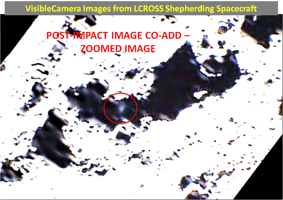
Within the ultraviolet/visible and near infra-red spectrometer and camera data was a faint, but distinct, debris plume created by the Centaur’s impact.

“There is a clear indication of a plume of vapor and fine debris,” said Colaprete. “Within the range of model predictions we made, the ejecta brightness appears to be at the low end of our predictions and this may be a clue to the properties of the material the Centaur impacted.”

The magnitude, form, and visibility of the debris plume add additional information about the concentrations and state of the material at the impact site.

From images and data, the team was able to determine the extent of the plume at 15 seconds after impact was approximately 6-8 km in diameter. Schultz said the Moon’s gravity pulled down most of ejecta within several minutes.

The LCROSS spacecraft also captured the Centaur impact flash in both mid-infrared (MIR) thermal cameras over a couple of seconds. The temperature of the flash provides valuable information about the composition of the material at the impact site. LCROSS also captured emissions and absorption spectra across the flash using an ultraviolet/visible spectrometer. Different materials release or absorb energy at specific wavelengths that are measurable by the spectrometers.

the locations of the Diviner LCROSS impact swaths overlain on a grayscale daytime thermal map of the Moon’s south polar region. Diviner data were used to help select the final LCROSS impact site inside Cabeus Crater, which sampled an extremely cold region in permanent shadow that can serve as an effective cold trap for water ice and other frozen volatiles. Credit NASA/GSFC/UCLA

Additionally, the Lunar Reconnaissance Orbiter’s Diviner instrument also obtained infrared observations of the LCROSS impact. LRO flew by the LCROSS Centaur impact site 90 seconds after impact at a distance of ~80 km. Both science teams are working together to analyze the their data.

The LCROSS spacecraft captured and returned data until virtually the last second before impact, Colaprete said, and the thermal and near-infrared cameras returned excellent images of the Centaur impact crater at a resolution of less than 6.5 feet (2 m).

“The images of the floor of Cabeus are exciting,” said Colaprete. “Being able to image the Centaur crater helps us reconstruct the impact process, which in turn helps us understand the observations of the flash and ejecta plume.”

Sources: LCROSS, LCROSS webcast

October 16, 2009December 24, 2015 by Fraser Cain

Satellite Finder

[/caption]
There are some amazing resources on the Internet that will let you track and find satellites in the sky. Did you know that the International Space Station is the brightest manmade object in the sky? It’s easy to see if you know when and were to look. So, this article should give you some good satellite finder resources, so you can track down and bag sightings of satellites.

The first place to start is NASA’s tracking page for the International Space Station, space shuttle and Hubble Space Telescope. This tells you where the spacecraft currently are, and also give you a way to find out when the spacecraft are going to be flying over your part of the world. They have a quick list of common locations, but you can also enter your latitude and longitude, and the system will give you some sighting opportunities.

Next, check out the Real Time Satellite Tracking page. This shows you the current position of thousands of satellites, and lets you see what’s overhead right now. You can set up satellite finders to watch the position of certain satellites. It’s an amazing resource.

Another great tool is Heaven’s Above. It lets you put in your local address, and then get predictions for satellites that will be overhead in the next few days. You can see the current position of the International Space Station, and much more.

If you have an iPhone, here’s a cool app that lets you find out the current location of the International Space Station and the space shuttle (if it’s in orbit right now).

If you have a satellite dish, and you need a satellite finder to maximize the strength of the signal, here’s a link to a Satellite finding kit from Amazon.com. It lets you finely tune the direction of your satellite dish to get the best signal from the satellite.

We have written many articles about satellites for Universe Today. Here’s an article about how you can watch satellites gather data in real time, and here’s a service that lets you launch your own satellite for only $8000.

We have done many episodes of Astronomy Cast about satellites. Listen to Episode 84: Getting Around the Solar System.

October 16, 2009April 26, 2016 by Tammy Plotner

Hot Crescent Rolls… A Bubble?

The Crescent Nebula by Dietmar Hager and Immo Gerber

[/caption]

The Crescent Nebula, also known as NGC 6888, is a very well renown and most intriguing object located in the constellation Cygnus in the northern hemisphere. At an apparent size of about 18 by 13 arc-minutes it is a very pale nebula. Even in a moderate amateur telescope you can’t quite see this one unless you have absolute dark skies (or narrow band filters) and a decent “light bucket”. So how do we get a chance to study it? Photographically, of course…

Spanning some 25 by 18 light years, gazing at NGC 6888 means we are looking 4700 years into the past, a past that renders a nebula fueled and excited by the blue star at the center. And not just any blue star – but a high mass super-giant star – one that depleted its fuel at “full speed”. Not only was it a super giant, but hot… in the class of “Wolf Rayet” stars (HD 192163). Now, after only a couple of million years the “stellar gas” is almost used up and the star is standing right before a significant change: a supernova candidate. Behold a star that vents its outer layers into space at terrific speed!

“Images are used to constrain models of the ionization structure of nebular features.” says Brian D. Moore (et al) of the Department of Physics and Astronomy, Arizona State University, “From these models, we infer physical conditions within features and estimate elemental abundances within the nebula. The results of our analysis, together with the degree of small-scale inhomogeneity apparent in the images, call into question the assumptions underlying traditional methodologies for interpretation of nebular spectroscopy. The thermal pressure of photoionized clumps is higher than the inferred internal pressure of the shocked stellar wind, implying that the current physical conditions have changed significantly over less than a few thousand years.”

While the central star sustains severe loss of mass, the gas is holding lots of oxygen and hydrogen… just before the individual big “bang” of the WR-star creating a “hot bubble” whose struture can’t quite be explained yet. “A detailed analysis of the H I distribution at low positive velocities allowed us to identify two different structures very probably related to the star and the ring nebula. From inside to outside they are: (1) an elliptical shell, 11.8×6.3 pc in size, that embraces the ring nebula (labeled inner shell); and (2) a distorted H I ring, 28 pc in diameter, also detected in IR emission (outer shell). The borders of the inner shell strikingly follows the brightest regions of NGC 6888, showing the sites where the interaction between the nebula and the surrounding gas occurs. A third structure, the external feature, is a broken arc detected at slightly higher velocities than the former shells.” says Christina Cappa (et al), “We propose a scenario in which the strong stellar wind of HD 192163, expanding in an inhomogeneous interstellar medium, blew the outer shell during the main sequence phase of the star. Later, the material ejected by the star during the LBV (or RSG) and WR phases created NGC 6888. This material encountered the innermost wall of the outer shell originating the inner shell. The association of the external feature with the star and the nebula is not clear.”

For a look inside, view the full size image!

Many thanks to Dietmar Hager and Immo Gerber of TAO-Observatory for sharing this incredible image!

October 16, 2009December 24, 2015 by Tammy Plotner

Request For Twilight Observations of U Scorpii

Further to AAVSO Alert Notice 367 and Special Notices 127 and 141, the AAVSO requests twilight observations of the recurrent nova U Scorpii prior to its solar conjunction in late 2009. These observations are in support of the long-term campaign by Dr. Bradley Schaefer (LSU) to catch this very fast nova during its rise.

AAVSO Special Notice #171: In 2008, the last ground-based observation of U Sco was made on 2008 November 2 (S. Kerr,
Glenlee, QLD, Australia). Observers are asked to do the best they can to observe U Sco as close to the Sun as possible. For this project, fainter-than observations are just as important as positive ones, and observers are asked to report all observations as promptly as possible via AAVSO WebObs.

For more information on the U Sco campaign and its science goals, please see the following URL: http://www.aavso.org/news/usco.shtml

U Sco is located at the following (J2000) coordinates:
RA:16:22:30.80, Dec: -17:52:43.0

Charts for U Sco may be plotted using AAVSO VSP: http://www.aavso.org/observing/charts/vsp/index.html?pickname=U%20Sco

(AAVSO Special Notice was prepared by M. Templeton)

Located north of Antares, U Scorpii is one of the most famous recurrent novae… and one of the fastest known. Able to shoot up to 8 or 9 magnitudes in less than 6 hours, dedicated observers are predicting that 2009 should see this cataclysmic variable star erupt with a vengeance. “I’ve calculated that the recurrent nova U Scorpii, north of Antares and east of the head of Scorpius, should explode any month now.” says Bradley E. Schaefer of Sky & Telescope, “My ‘crystal ball’ is based on old archival photographs and data from amateur astronomers. This brings a golden opportunity for amateurs and professionals to catch the early hours of a nova eruption and to prepare in advance for an intensive observing campaign.”

While professional observatories and NASA’s Swift Satellite will be busy gathering information about any possible eruption, there’s more than enough room for amateur observations. While it’s great to have modern equipment and credited astronomers to capture the action, their eyes can’t watch 24/7 – and chances are good that any outburst may very well be captured by ordinary viewers working in the field. “Amateurs provided essentially the whole light curves for the last three eruptions.” says Brad, “Now, with some advance warning to allow preparations, and with a little luck, the upcoming eruption of U Sco could produce the best record of a nova outburst — of any kind — ever.”

Please promptly report all observations to the AAVSO with the name “U SCO”.

October 16, 2009December 24, 2015 by Tammy Plotner

Weekend SkyWatcher’s Forecast – October 16-18, 2009

[/caption]

Greetings, fellow Stargazers! Were you up early this morning? If so, you were greeted by an awesome scene, much like this one captured by Danilo Pivato. There’s nothing more eyecatching the a close appearance of Venus and the Moon! With dark skies this weekend, it will be a good opportunity to broaden your astronomical horizons by chasing lesser known objects in both binoculars and telescopes. Of course there are challenges, too! Whenever you’re ready, I’ll see you in the back yard….

Friday, October 16 – Celestial scenery alert! Be up and outside this morning before dawn. The incredible duo of Venus and Saturn will be joined by the Moon! In 1982, the 30th return of Halley’s Comet was observed with the 5-meter (20000) Hale Telescope at the Mount Palomar Observatory. The comet was beyond the orbit of Saturn!

Tonight let’s head toward the region of Cas A and see what we can find. Although Cas A is itself not visible in amateur equipment, it is known to be associated with a 10,000-light-year-distant supernova remnant related to an unnoticed event occurring more than 300 years ago. The remnant itself has now expanded to a region filling some 10 light-years of space and has been imaged using orbiting X-ray observatories.

The closest deep-sky study to Cas A is the dense and compact open cluster NGC 7510 (RA 23 11 00 Dec +60 34 00). This diminutive, magnitude 7.9 study can just be glimpsed as a hazy patch in large binoculars and small scopes, with a few of its brightest 10th magnitude members resolvable at higher magnifications. Doubling the aperture brings out a dozen or so of NGC 7510’s 12th magnitude stars against the teeming glow of numerous fainter members. Double the aperture again, and 60 stars to magnitude 14 are possible. Many amateurs have discovered that the combination of a small rich field refractor, a 600 apochromatic refractor, and a 1200 Newtonian makes for the ultimate in observing equipment. But don’t forget those binoculars!

Saturday, October 17 – Today we mark the birth of Dr. Mae C. Jemison, the first black woman to go into space! Tonight let’s revisit M39 and use it as our touchstone to seek out other deep-sky gems. Starting with M39, head less than two finger-widths east-southeast (RA 21 53 32 Dec +47 16 06) to a 7.2 magnitude open cluster, one associated with the 12th magnitude ‘‘Cocoon Nebula.’’

Collectively known as IC 5146, this cluster with nebulosity consists largely of 12th magnitude stars and is just about mid-sized. Barely detectable in a small scope, this 4,000-light-year-distant cluster needs aperture to come out and play. Large scopes may make seeing the nebula possible, although an appropriate filter may be necessary from most observing sites. To assist in finding the Cocoon, look for the stream of the dark obscuration nebula B168 touching its eastern frontier.

Returning again to M39, head two finger-widths southwest in the direction of Deneb to seek 6.8 magnitude IC 1369 (RA 21 12 06 Dec +47 44 00). Mid-sized instruments will show a dozen or so 12th and 13th magnitude members within a misty haze of those waiting to be resolved. Also known as alternative catalog study Pechue (AN 3259), IC 1369 has been studied for luminosity features.

Sunday, October 18, 2009 – Tonight it’s a New Moon! Time to break out the muscle and challenge big telescope users to hone their skills. It’s galaxy-hunting time, and our destination for tonight is the Hickson Compact Group 87 (RA 20 48 11 Dec -19 50 24).

Several billion years ago, on the ecliptic plane about 4 degrees west/southwest of Theta Capricorni, and around 400 million light-years from our Solar System, a galactic association decided to form its own ‘‘Local Group.’’ Orbiting around a common center every 100 million years, their mutual gravity is pulling each of them apart, creating starbursts and feeding their active galactic nuclei. Small wonder they’re shredding each other. They’re only 170,000 light-years apart! One day HCG 87 may even form a single elliptical galaxy bright enough for the average telescope to see, but as they are now, this group isn’t going to be seen with anything less than 20 inch aperture.

So, shall we try something a little more within the realm of reality? Then go ahead and drop about 8 degrees south of Theta, and try picking up on the NGC7016/17/18 group (RA 21 07 20 Dec -25 29 15). Are they faint? Of course! It wouldn’t be a challenge if they were easy, would it? With an average magnitude of 14, this tight trio known as Leavenworth 1 is around 600 million light-years away. They’re very small and not very easy to locate, but for those who like something a bit different, give it a try!

Until next week? Dreams really do come true when you keep on reaching for the stars!

This week’s awesome images are (in order of appearance): The Moon and Venus: Courtesy of Danilo Pivato of Northern Galactic, NGC 7510, IC 5146, IC 1369, Hickson Compact Group 87 and NGC 7016/17/18 (credit—Palomar Observatory, courtesy of Caltech). We thank you so much!

October 16, 2009December 24, 2015 by Nancy Atkinson

Where Could Humans Survive in our Solar System?

Habitability in our solar system. Credit: UPR Arecibo, NASA PhotoJournal

[/caption]
If humans were forced to vacate Earth, where is the next best place in our solar system for us to live? A study by the University of Puerto Rico at Arecibo has provided a quantitative evaluation of habitability to identify the potential habitats in our solar system. Professor Abel Mendez, who produced the study also looked at how the habitability of Earth has changed in the past, finding that some periods were even better than today.

Mendez developed a Quantitative Habitability Theory to assess the current state of terrestrial habitability and to establish a baseline for relevant comparisons with past or future climate scenarios and other planetary bodies including extrasolar planets.

“It is surprising that there is no agreement on a quantitative definition of habitability,” said Mendez, a biophysicist. “There are well-established measures of habitability in ecology since the 1970s, but only a few recent studies have proposed better alternatives for the astrobiology field, which is more oriented to microbial life. However, none of the existing alternatives from the fields of ecology to astrobiology has demonstrated a practical approach at planetary scales.”

His theory is based on two biophysical parameters: the habitability (H), as a relative measure of the potential for life of an environment, or habitat quality, and the habitation (M), as a relative measure of biodensity, or occupancy. Within the parameters are physiological and environmental variables which can be used to make predictions about the distribution, and abundance of potential food (both plant and microbial life), environment and weather.

The image above shows a comparison of the potential habitable space available on Earth, Mars, Europa, Titan, and Enceladus. The green spheres represent the global volume with the right physical environment for most terrestrial microorganisms. On Earth, the biosphere includes parts of the atmosphere, oceans, and subsurface (here’s a biosphere definition). The potential global habitats of the other planetary bodies are deep below their surface.

Enceladus has the smallest volume but the highest habitat-planet size ratio followed by Europa. Surprisingly, Enceladus also has the highest mean habitability in the Solar System, even though it is farther from the sun, and Earth, making it harder to get to. Mendez said Mars and Europa would be the best compromise between potential for life and accessibility.

n Oct. 5, 2008. Image credit: NASA/JPL/Space Science Institute Cassini came within 25 kilometers (15.6 miles) of the surface of Enceladus o

“Various planetary models were used to calculate and compare the habitability of Mars, Venus, Europa, Titan, and Enceladus,” Mendez said. “Interestingly, Enceladus resulted as the object with the highest subsurface habitability in the solar system, but too deep for direct exploration. Mars and Europa resulted as the best compromise between habitability and accessibility. In addition, it is also possible to evaluate the global habitability of any detected terrestrial-sized extrasolar planet in the future. Further studies will expand the habitability definition to include other environmental variables such as light, carbon dioxide, oxygen, and nutrients concentrations. This will help expand the models, especially at local scales, and thus improve its application in assessing habitable zones on Earth and beyond.”

Studies about the effects of climate change on life are interesting when applied to Earth itself. “The biophysical quantity Standard Primary Habitability (SPH) was defined as a base for comparison of the global surface habitability for primary producers,” Mendez said. “The SPH is always an upper limit for the habitability of a planet but other factors can contribute to lower its value. The current SPH of our planet is close to 0.7, but it has been up to 0.9 during various paleoclimates, such as during the late Cretaceous period when the dinosaurs went extinct. I’m now working on how the SPH could change under global warming.”

The search for habitable environments in the universe is one of the priorities of the NASA Astrobiology Institute and other international organizations. Mendez’s studies also focus on the search for life in the solar system, as well as extrasolar planets.

“This work is important because it provides a quantitative measure for comparing habitability,” said NASA planetary scientists Chris McKay. “It provides an objective way to compare different climate and planetary systems.”

“I was pleased to see Enceladus come out the winner,” McKay said. “I’ve thought for some time that it was the most interesting world for astrobiology in the solar system.”

Mendez presented his results at the Division for Planetary Sciences of the American Astronomical Society meeting earlier this month.

Source: AAS DPS

October 15, 2009January 24, 2021 by Nancy Atkinson

Amazing and Marvelous Mars Dunes

Sand dunes on Mars from MRO's HiRISE camera. Credit: NASA/JPL University of Arizona

[/caption]
I see the Bad Astronomer has beat me to the punch by posting this image before I could. But what an amazing and gorgeous image of dunes on Mars! However, my initial thought when I saw this on the HiRISE webpage was perhaps this was the first long-awaited look at Phil’s tattoo. Seriously, doesn’t this look like it could be body art? The dunes even have a Phil-like flesh color. But this wonderful image was taken by the HiRISE camera on the Mars Reconnaissance Orbiter. There is a great database of dune images gathered for the US Geological Survey on the HiRISE website, and below, take a gander at more lovely dune images:

Click on each image to learn more from the HiRISE website.

Russell Crater dunes. Credit: Credit: NASA/JPL/University of Arizona

Dunes in the Western Nereidum Montes. Credit: NASA/JPL University of Arizona

Sand dunes. Credit: NASA/JPL/University of Arizona

Dark dunes. Credit: NASA/JPL/University of Arizona

Check out the HiRISE website for more great images from Mars!

October 15, 2009December 24, 2015 by Fraser Cain

Satellite Map

[/caption]
There are thousands of satellites overhead in space right now, and many of them are being used to map every single square meter of planet Earth. And many of these images are being freely distributed on the Internet so you can access them through any browser. If you’re looking for a satellite map, there are many services out there that can help you out.

Probably the easiest and best place to start is with the Google Maps service from Google. This allows you to see a satellite map of the entire Earth. You can drag around the map to browse around the planet, and you can zoom out and in right down to the highest resolution images they have in their server. In many cases this means you can see your house, your yard, and even your car parked out in the street. You can also type in a specific address location and go straight there. There are street maps you can overlay or remove, you can get driving directions, and much more. And the Google Maps API has been made available by Google to other websites, so people are developing mashups that let you track running routes and find the nearest bathroom.

An even cooler satellite mapping service is Google Earth. Unlike Google Maps, you have to download Google Earth to your local PC, Mac or Linux machine (there’s even an iPhone version). Then you get this cool spinning 3-D version of the Earth. You can zoom out and in, type in a specific location address or geocode to find any spot on Earth. They also have a big library of additional layers that you can put over top, to see additional information mapped on the Earth. It’s well worth the download.

Another good service is TerraServer; they let you buy satellite maps if you want a nice printed version for your wall. If you don’t want to use Google, there are similar mapping tools from Microsoft and Yahoo.

We have written many articles about how satellites are being used to map the Earth. Here’s an article about how scientists use satellite photos to track penguin poop from space, and how Google’s maps had a satellite view of Obama’s inauguration.

We have also recorded an episode of Astronomy Cast all about Earth. Listen here, Episode 51: Planet Earth.

October 15, 2009December 24, 2015 by Nancy Atkinson

Spacecraft Detects Mysterious “Ribbon” at Edge of Solar System

Accurate timing of the incoming ENAs allows the IBEX team to obtain a higher resolution in the latitudinal direction. The inset at right shows some of the fine detail of the ribbon. Credit: Southwest Research Institute (SwRI)

[/caption]

Since it launched a year ago, the Interstellar Boundary Explorer (IBEX) has been monitoring heliosphere and how our Sun interacts with and the local interstellar medium — the gas and dust trapped in the vacuum of space. The first results from the mission, combined with data from the Cassini mission, are showing the heliosphere to be different from what researchers have previously thought. Data show an unexpected bright band or ribbon of surprisingly high-energy emissions. “We knew there would be energetic neutral atoms coming in from the very edge of the heliosphere, and our theories said there would be small variations in their emissions,” said David McComas, IBEX Principal Investigator at a press conference on Thursday. “But instead we are seeing two-to-three hundred percent variations, and this is not entirely understood. Whatever we thought about this before is definitely not right.”

The energies IBEX has observed range from 0.2 to 6.0 kiloelectron volts, and the scientists said its flux is two to three times greater than the ENA activity throughout the rest of the heliosphere. McComas and his colleagues said that no existing model can explain all the dominant features of this “ribbon.” Instead, they suggest that these new findings will prompt a change in our understanding of the heliosphere and the processes that shape it.

This image illustrates one possible explanation for the bright ribbon of emission seen in the IBEX map. The galactic magnetic field shapes the heliosphere as it drapes over it. The ribbon appears to trace the area where the magnetic field is most parallel to the surface of the heliosphere (the heliopause). Credit: Southwest Research institute

McComas suggested that the energetic neutral atom (ENA) ribbon could be caused by interactions between the heliosphere and the local interstellar magnetic field. “The local interstellar magnetic field is oriented in such a way that it correlates with the ribbon. If you ‘paint’ the ribbon on the boundary of the heliosphere, the magnetic field is like big bungie cords that pushing in along the sides and at southern part of the heliosphere. Somehow the magnetic field seems to be playing a dominant roll in these interactions, but we don’t know it could produced these higher fluxes. We have to figure out what physics were are missing.”

The solar wind streaks away from the sun in all directions at over a millions kilometers per hour. It creates a bubble in space around our solar system.

For the first ten billion kilometers of its radius, the solar wind travels at over a million kilometers per hour. It slows as it begins to collide with the interstellar medium, and the point where the solar wind slows down is the termination shock; the point where the interstellar medium and solar wind pressures balance is called the heliopause; the point where the interstellar medium, traveling in the opposite direction, slows down as it collides with the heliosphere is the bow shock.

The Voyager spacecraft have explored this region, but didn’t detect the ribbon. Team member Eric Christian said the ribbon wound in between the location of Voyager 1 and 2, and they couldn’t detect it in their immediate areas. Voyager 1 spacecraft encountered the helioshock in 2004 when it reached the region where the charged particles streaming off the sun hit the neutral gas from interstellar space. Voyager 2 followed into the solar system’s edge in 2007. While these spacecraft made the first explorations of this region, IBEX is now revealing a a more complete picture, filling in where the Voyagers couldn’t. Christian compared Voyager 1 and 2 to be like weather stations while IBEX is first weather satellite to provide more complete coverage.

McComas said his first reaction when the data started coming in was that of terror because he thought something must be wrong with the spacecraft. But as more data kept coming back each week, the team realized that they were wrong, and the spacecraft was right.

“Our next steps will be to go through all the detailed observations and rack them up against the various models and go find what it is that we are missing, what we’ve been leaving out,” he said.

For more information and visuals, see this NASA webpage.

October 15, 2009December 24, 2015 by Nancy Atkinson

If We Live in a Multiverse, How Many Are There?

[/caption]
Theoretical physics has brought us the notion that our single universe is not necessarily the only game in town. Satellite data from WMAP, along with string theory and its 11- dimensional hyperspace idea has produced the concept of the multiverse, where the Big Bang could have produced many different universes instead of a single uniform universe. The idea has gained popularity recently, so it was only a matter of time until someone asked the question of how many multiverses could possibly exist. The number, according to two physicists, could be “humongous.”

Andrei Linde and Vitaly Vanchurin at Stanford University in California, did a few back-of- the- envelope calculations, starting with the idea that the Big Bang was essentially a quantum process which generated quantum fluctuations in the state of the early universe. The universe then underwent a period of rapid growth called inflation during which these perturbations were “frozen,” creating different initial classical conditions in different parts of the cosmos. Since each of these regions would have a different set of laws of low energy physics, they can be thought of as different universes.

Linde and Vanchurin then estimated how many different universes could have appeared as a result of this effect. Their answer is that this number must be proportional to the effect that caused the perturbations in the first place, a process called slow roll inflation, — the solution Linde came up with previously to answer the problem of the bubbles of universes colliding in the early inflation period. In this model, inflation occurred from a scalar field rolling down a potential energy hill. When the field rolls very slowly compared to the expansion of the universe, inflation occurs and collisions end up being rare.

Using all of this (and more – see their paper here) Linde and Vanchurin calculate that the number of universes in the multiverse and could be at least 10^10^10^7, a number which is definitely “humungous,” as they described it.

The next question, then, is how many universes could we actually see? Linde and Vanchurin say they had to invoke the Bekenstein limit, where the properties of the observer become an important factor because of a limit to the amount of information that can be contained within any given volume of space, and by the limits of the human brain.

The total amount of information that can be absorbed by one individual during a lifetime is about 10^16 bits. So a typical human brain can have 10^10^16 configurations and so could never distinguish more than that number of different universes.

The number of multiverses the human brain could distinguish. Credit: Linde and Vanchurin

“So, the total number of possibilities accessible to any given observer is limited not only by the entropy of perturbations of metric produced by inflation and by the size of the cosmological horizon, but also by the number of degrees of freedom of an observer,” the physicists write.

“We have found that the strongest limit on the number of different locally distinguishable geometries is determined mostly by our abilities to distinguish between different universes and to remember our results,” wrote Linde and Vanchurin. “Potentially it may become very important that when we analyze the probability of existencse of a universe of a given type, we should be talking about a consistent pair: the universe and an observer who makes the rest of the universe “alive” and the wave function of the rest of the universe time-dependant.”

So their conclusion is that the limit does not depend on the properties of the multiverse itself, but on the properties of the observer.

They hope to further study this concept to see if this probability if proportional to the observable entropy of inflation.

Sources: ArXiv, Technology Review Blog